Computer Vision: Models, Learning, and Inference (2012)

The most common representation for uncertainty in machine vision is the multivariate normal distribution. We devote this chapter to exploring its main properties, which will be used extensively throughout the rest of the book.

Recall from Chapter 3 that the multivariate normal distribution has two parameters: the mean μ and covariance ∑. The mean μ is a D × 1 vector that describes the position of the distribution. The covariance ∑ is a symmetric D × Dpositive definite matrix (implying that z^T∑z is positive for any real vector z and describes the shape of the distribution. The probability density function is

or for short

5.1 Types of covariance matrix

Covariance matrices in multivariate normals take three forms, termed spherical, diagonal, and full covariances. For the two-dimensional (bivariate) case, these are

The spherical covariance matrix is a positive multiple of the identity matrix and so has the same value on all of the diagonal elements and zeros elsewhere. In the diagonal covariance matrix, each value on the diagonal has a different positive value. The full covariance matrix can have nonzero elements everywhere although the matrix is still constrained to be symmetric and positive definite so for the 2D example, σ²₁₂ = σ²₂₁.

For the bivariate case (Figure 5.1), spherical covariances produce circular iso-density contours. Diagonal covariances produce ellipsoidal iso-contours that are aligned with the coordinate axes. Full covariances also produce ellipsoidal iso-density contours, but these may now take an arbitrary orientation. More generally, in D dimensions, spherical covariances produce iso-contours that are D-spheres, diagonal covariances produce iso-contours that are D-dimensional ellipsoids aligned with the coordinate axes, and full covariances produce iso-contour that are D-dimensional ellipsoids in general position.

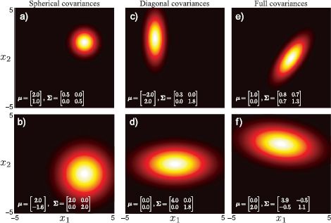
Figure 5.1 Covariance matrices take three forms. a-b) Spherical covariance matrices are multiples of the identity. The variables are independent and the iso-probability surfaces are hyperspheres. c-d) Diagonal covariance matrices permit different nonzero entries on the diagonal, but have zero entries elsewhere. The variables are independent, but scaled differently and the isoprobability surfaces are hyperellipsoids (ellipses in 2D) whose principal axes are aligned to the coordinate axes. e-f) Full covariance matrices are symmetric and positive definite. Variables are dependent, and iso-probability surfaces are ellipsoids that are not aligned in any special way.

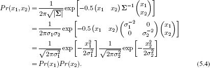
When the covariance is spherical or diagonal, the individual variables are independent. For example, for the bivariate diagonal case with zero mean, we have

5.2 Decomposition of covariance

We can use the foregoing geometrical intuitions to decompose the full covariance matrix ∑_full. Given a normal distribution with mean zero and a full covariance matrix, we know that the iso-contours take an ellipsoidal form with the major and minor axes at arbitrary orientations.

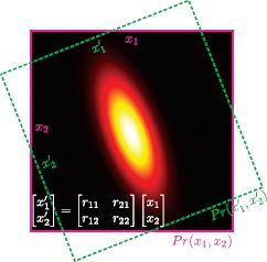
Figure 5.2 Decomposition of full covariance. For every bivariate normal distribution in variables x₁ and x₂ with full covariance matrix, there exists a coordinate system with variables x′₁ and x′₂ where the covariance is diagonal: the ellipsoidal iso-contours align with the coordinate axes x′₁ and x′₂ in this canonical coordinate frame. The two frames of reference are related by the rotation matrix R which maps (x′₁, x′₂) to (x₁, x₂). From this it follows (see text) that any covariance matrix ∑ can be broken down into the product R^T∑′_diagR of a rotation matrix R and a diagonal covariance matrix ∑′_diag.

Now consider viewing the distribution in a new coordinate frame where the axes that are aligned with the axes of the normal (Figure 5.2): in this new frame of reference, the covariance matrix ∑′_diag will be diagonal. We denote the data vector in the new coordinate system by x′ = [x′₁, x′₂]^T where the frames of reference are related by x′ = Rx. We can write the probability distribution over x′ as

We now convert back to the original axes by substituting in x′ = Rx to get

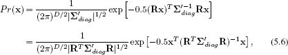
where we have used |R^T∑′R| = |R^T|.|∑′|.|R| = 1.|∑′|.1 = |∑′|. Equation 5.6 is a multivariate normal with covariance

We conclude that full covariance matrices are expressible as a product of this form involving a rotation matrix R and a diagonal covariance matrix ∑′_diag. Having understood this, it is possible to retrieve these elements from an arbitrary valid covariance matrix ∑_full by decomposing it in this way using the singular value decomposition.

The matrix R contains the principal directions of the ellipsoid in its columns. The values on the diagonal of ∑′_diag encode the variance (and hence the width of the distribution) along each of these axes. Hence we can use the results of the singular value decomposition to answer questions about which directions in space are most and least certain.

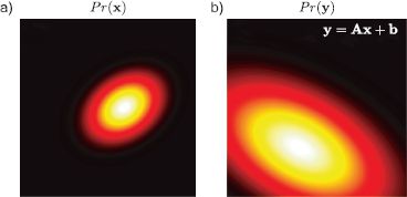
Figure 5.3 Transformation of normal variables. a) If x has a multivariate normal pdf and we apply a linear transformation to create new variable y = Ax + b, then b) the distribution of y is also multivariate normal. The mean and covariance of y depend on the original mean and covariance of x and the parameters A and b.

5.3 Linear transformations of variables

The form of the multivariate normal is preserved under linear transformations y = Ax + b (Figure 5.3). If the original distribution was

then the transformed variable y is distributed as

This relationship provides a simple method to draw samples from a normal distribution with mean μ and covariance ∑. We first draw a sample x from a standard normal distribution (with mean μ = 0 and covariance ∑ = I) and then apply the transformation y = ∑^1/2x + μ.

5.4 Marginal distributions

If we marginalize over any subset of random variables in a multivariate normal distribution, the remaining distribution is also normally distributed (Figure 5.4). If we partition the original random variable into two parts x = [x^T₁, x^T₂]^T so that

then

So, to find the mean and covariance of the marginal distribution of a subset of variables, we extract the relevant entries from the original mean and covariance.

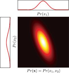
Figure 5.4 The marginal distribution of any subset of variables in a normal distribution is also normally distributed. In other words, if we sum over the distribution in any direction, the remaining quantity is also normally distributed. To find the mean and the covariance of the new distribution, we can simply extract the relevant entries from the original mean and covariance matrix.

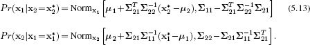
5.5 Conditional distributions

If the variable x is distributed as a multivariate normal, then the conditional distribution of a subset of variables x₁ given known values for the remaining variables x₂ is also distributed as a multivariate normal (Figure 5.5). If

then the conditional distributions are

5.6 Product of two normals

The product of two normal distributions is proportional to a third normal distribution (Figure 5.6). If the two original distributions have means a and b and covariances A and B, respectively, then we find that

where the constant κ is itself a normal distribution,

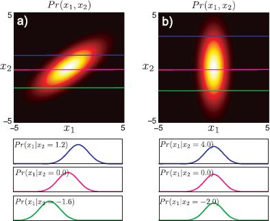
Figure 5.5 Conditional distributions of multivariate normal. a) If we take any multivariate normal distribution, fix a subset of the variables, and look at the distribution of the remaining variables, this distribution will also take the form of a normal. The mean of this new normal depends on the values that we fixed the subset to, but the covariance is always the same. b) If the original multivariate normal has spherical or diagonal covariance, both the mean and covariance of the resulting normal distributions are the same, regardless of the value we conditioned on: these forms of covariance matrix imply independence between the constituent variables.

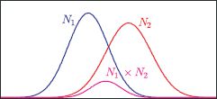
Figure 5.6 The product of any two normals N₁ and N₂ is proportional to a third normal distribution, with a mean between the two original means and a variance that is smaller than either of the original distributions.

5.6.1 Self-conjugacy

The preceding property can be used to demonstrate that the normal distribution is self-conjugate with respect to its mean μ. Consider taking a product of a normal distribution over data x and a second normal distribution over the mean vector μ of the first distribution. It is easy to show from Equation 5.14 that

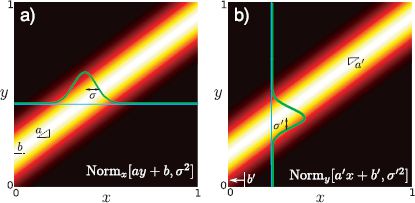
Figure 5.7 a) Consider a normal distribution in x whose variance σ² is constant, but whose mean is a linear function ay + b of a second variable y. b) This is mathematically equivalent to a constant κ times a normal distribution in y whose variance σ^′2 is constant and whose mean is a linear function a′ x + b′ of x.

which is the definition of conjugacy (see Section 3.9). The new parameters and are determined from Equation 5.14. This analysis assumes that the variance ∑ is being treated as a fixed quantity. If we also treat this as uncertain, then we must use a normal inverse Wishart prior.

5.7 Change of variable

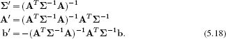
Consider a normal distribution in variable x whose mean is a linear function Ay + b of a second variable y. We can reexpress this in terms of a normal distribution in y, which is a linear function A′x + b′ of x so that

where κ is a constant and the new parameters are given by

This relationship is mathematically opaque, but it is easy to understand visually when x and y are scalars (Figure 5.7). It is often used in the context of Bayes’ rule where our goal is to move from Pr(x|y) to Pr(y|x).

Summary

In this chapter we have presented a number of properties of the multivariate normal distribution. The most important of these relates to the marginal and conditional distributions: when we marginalize or take the conditional distribution of a normal with respect to a subset of variables, the result is another normal. These properties are exploited in many vision algorithms.

Notes

The normal distribution has further interesting properties which are not discussed because they are not relevant for this book. For example, the convolution of a normal distribution with a second normal distribution produces a function that is proportional to a third normal, and the Fourier transform of a normal profile creates a normal profile in frequency space. For a different treatment of this topic the interested reader can consult Chapter 2 of Bishop (2006).

Problems

5.1 Consider a multivariate normal distribution in variable x with mean μ and covariance ∑. Show that if we make the linear transformation y = Ax + b, then the transformed variable y is distributed as

5.2 Show that we can convert a normal distribution with mean μ and covariance ∑ to a new distribution with mean 0 and covariance I using the linear transformation y = Ax + b where

This is known as the whitening transformation.

5.3 Show that for multivariate normal distribution

the marginal distribution in x₁ is

Hint: Apply the transformation y = [I, 0]x.

5.4 The Schur complement identity states that inverse of a matrix in terms of its subblocks is

Show that this relation is true.

5.5 Prove the conditional distribution property for the normal distribution: if

then

Hint: Use Schur’s complement.

5.6 Use the conditional probability relation for the normal distribution to show that the conditional distribution Pr(x₁|x₂ = k) is the same for all k when the covariance is diagonal and the variables are independent (see Figure 5.5b).

5.7 Show that

5.8 For the 1D case, show that when we take the product of the two normal distributions with means μ₁, μ₂ and variances σ₁², σ₂² the new mean lies between the original two means and the new variance is smaller than either of the original variances.

5.9 Show that the constant of proportionality κ in the product relation in Problem 5.7 is also a normal distribution where

5.10 Prove the change of variable relation. Show that

and derive expressions for κ, A′, b′, and ∑′. Hint: Write out the terms in the original exponential, extract quadratic and linear terms in y, and complete the square.