Computer Vision: Models, Learning, and Inference (2012)

Part II

Machine learning for machine vision

Chapter 7

Modeling complex data densities

In the last chapter we showed that classification with generative models is based on building simple probability models. In particular, we build class-conditional density functions Pr(x|w = k) over the observed data x for each value of the world state w.

In Chapter 3 we introduced several probability distributions that could be used for this purpose, but these were quite limited in scope. For example, it is not realistic to assume that all of the complexities of visual data are well described by the normal distribution. In this chapter, we show how to construct complex probability density functions from elementary ones using the idea of a hidden variable.

As a representative problem we consider face detection we observe a 60 × 60 RGB image patch, and we would like to decide whether it contains a face or not. To this end, we concatenate the RGB values to form the 10800 × 1 vector x. Our goal is to take the vector x and return a label w ∈ {0, 1} indicating whether it contains background (w = 0) or a face (w = 1). In a real face detection system, we would repeat this procedure for every possible subwindow of an image (Figure 7.1).

We will start with a basic generative approach in which we describe the likelihood of the data in the presence/absence of a face with a normal distribution. We will then extend this model to address its weaknesses. We emphasize though that state-of-the-art face detection algorithms are not based on generative methods such as these; they are usually tackled using the discriminative methods of Chapter 9. This application was selected for purely pedagogical reasons.

7.1 Normal classification model

We will take a generative approach to face detection; we will model the probability of the data x and parameterize this by the world state w. We will describe the data with a multivariate normal distribution so that

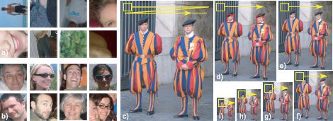
Figure 7.1 Face detection. Consider examining a small window of the image (here 60 × 60). We concatenate the RGB values in the window to make a data vector x of dimension 10800 × 1. The goal of face detection is to infer a label w ∈ {0, 1} indicating whether the window contains a) a background region (w = 0) or b) an aligned face (w = 1). c–i) We repeat this operation at every position and scale in the image by sweeping a fixed size window through a stack of resized images, estimating w at every point.

or treating the two possible values of the state w separately, we can explicitly write

These expressions are examples of class conditional density functions. They describe the density of the data x conditional on the value of the world state w.

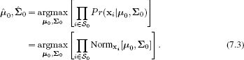
The goal of learning is to estimate the parameters θ = {μ₀, Σ₀, μ₁, Σ₁} from example pairs of training data {x_i, w_i}^I_i=1. Since parameters μ₀ and Σ₀ are concerned exclusively with background regions (where w = 0), we can learn them from the subset of training data ₀ that belonged to the background. For example, using the maximum likelihood approach, we would seek

Similarly, μ₁ and Σ₁ are concerned exclusively with faces (where w = 1) and can be learned from the subset ₁ of training data which contained faces. Figure 7.2 shows the maximum likelihood estimates of the parameters where we have used the diagonal form of the covariance matrix.

The goal of the inference algorithm is to take a new facial image x and assign a label w to it. To this end, we define a prior over the values of the world state Pr(w) = Bern_w[λ] and apply Bayes’ rule.

All of these terms are simple to compute, and so inference is very easy and will not be discussed further in this chapter.

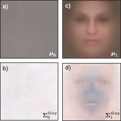
Figure 7.2 Class conditional density functions for normal model with diagonal covariance. Maximum likelihood fits based on 1000 training examples per class. a) Mean for background data μ₀ (reshaped from 10800 × 10800 × 1 vector to 60 × 60 RGB image). b) Reshaped square root of diagonal covariance for background data Σ₀. c) Mean for face data μ₁. d) Covariance for face data Σ₁. The background model has little structure: the mean is uniform, and the variance is high everywhere. The mean of the face model clearly captures class-specific information. The covariance of the face is larger at the edges of the image, which usually contain hair or background.

7.1.1 Deficiencies of the multivariate normal model

Unfortunately, this model does not detect faces reliably. We will defer presenting experimental results until Section 7.9.1, but for now please take it on trust that while this model achieves above-chance performance, it doesn’t come close to producing a state-of-the-art result. This is hardly surprising: the success of this classifier hinges on fitting the data with a normal distribution. Unfortunately, this fit is poor for three reasons (Figure 7.3).

• The normal distribution is unimodal; neither faces nor background regions are well represented by a pdf with a single peak.

• The normal distribution is not robust; a single outlier can dramatically affect the estimates of the mean and covariance.

• The normal distribution has too many parameters; here the data have D = 10800 dimensions. The full covariance matrix contains D(D + 1)/2 parameters. With only 1000 training examples, we cannot even specify these parameters uniquely, so we were forced to use the diagonal form.

We devote the rest of this chapter to tackling these problems. To make the density multimodal, we introduce mixture models. To make the density robust, we replace the normal with the t-distribution. To cope with parameter estimation in high dimensions, we introduce subspace models.

The new models have much in common with each other. In each case, we introduce a hidden or latent variable h_i associated with each observed data point x_i. The hidden variable induces the more complex properties of the resulting pdf. Moreover, because the structure of the models is similar, we can use a common approach to learn the parameters.

In the following section, we present an abstract discussion of how hidden variables can be used to model complex pdfs. In Section 7.3, we discuss how to learn the parameters of models with hidden variables. Then in Sections 7.4, 7.5, and 7.6, we will introduce mixture models, t-distributions, and factor analysis, respectively.

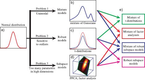
Figure 7.3 a) Problems with the multivariate normal density. b) Normal models are unimodal, but mixtures of Gaussians can model multimodal distributions. c) Normal distributions are not robust to outliers, but t-distributions can cope with unusual observations. d) Normal models need many parameters in high dimensions but subspace models reduce this requirement. e) These solutions can be combined to form hybrid models addressing several of these problems at once.

7.2 Hidden variables

To model a complex probability density function over the variable x, we will introduce a hidden or latent variable h, which may be discrete or continuous. We will discuss the continuous formulation, but all of the important concepts transfer to the discrete case.

To exploit the hidden variables, we describe the final density Pr(x) as the marginalization of the joint density Pr(x, h) between x and h so that

We now concentrate on describing the joint density Pr(x, h). We can choose this so that it is relatively simple to model but produces an expressive family of marginal distributions Pr(x) when we integrate over h (see Figure 7.4).

Whatever form we choose for the joint distribution, it will have some parameters θ, and so really we should write

There are two possible approaches to fitting the model to training data {x_i}^I_i=1 using the maximum likelihood method. We could directly maximize the log likelihood of the distribution Pr(x) from the left-hand side of Equation 7.6so that

This formulation has the advantage that we don’t need to involve the hidden variables at all. However, in the models that we will consider, it will not result in a neat closed form solution. Of course, we could apply a brute force nonlinear optimization technique (Appendix B), but there is an alternative approach: we use the expectation maximization algorithm, which works directly with the right-hand side of Equation 7.6 and seeks

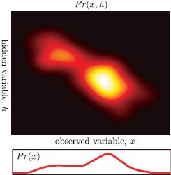
Figure 7.4 Using hidden variables to help model complex densities. One way to model the density Pr(x) is to consider the joint probability distribution Pr(x, h) between the observed data x and a hidden variable h. The density Pr(x) can be considered as the marginalization of (integral over) this distribution with respect to the hidden variable h. As we manipulate the parameters θ of this joint distribution, the marginal distribution changes and the agreement with the observed data {x_i}^I_i=1 increases or decreases. Sometimes it is easier to fit the distribution in this indirect way than to directly manipulate Pr(x).

7.3 Expectation maximization

In this section, we will present a brief description of the expectation maximization (EM) algorithm. The goal is to provide just enough information to use this technique for fitting models. We will return to a more detailed treatment in Section 7.8.

The EM algorithm is a general-purpose tool for fitting parameters θ in models of the form of Equation 7.6 where

The EM algorithm works by defining a lower bound [{q_i(h_i)}, θ] on the log likelihood in Equation 7.9 and iteratively increasing this bound. The lower bound is simply a function that is parameterized by θ and some other quantities and is guaranteed to always return a value that is less than or equal to the log likelihood L[θ] for any given set of parameters θ (Figure 7.5).

For the EM algorithm, the particular lower bound chosen is

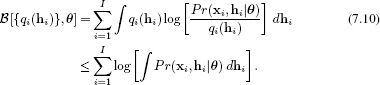
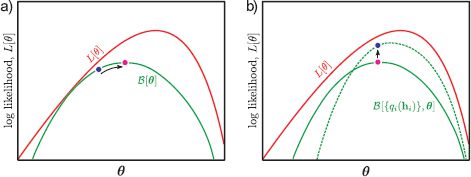
Figure 7.5 Manipulating the lower bound. a) Consider the log likelihood L[θ] of the data {x}^I_i=1 as a function of the model parameters θ (red curve). In maximum likelihood learning, our goal is to find the parameters θ that maximize this function. A lower bound on the log likelihood is another function [θ] of the parameters θ that is everywhere lower or equal to the log likelihood (green curve). One way to improve the current estimate (blue dot) is to manipulate the parameters so that [θ] increases (pink dot). This is the goal of the maximization step of the EM algorithm. b) The lower bound [{q_i (h_i)}, θ] also depends on a set of probability distributions {q_i(h_i)}^I_i=1 over hidden variables {h_i}. Manipulating these probability distributions changes the value that the lower bound returns for every θ (e.g., green curve). So a second way to improve the current estimate (pink dot) is to change the distributions in such a way that the curve increases for the current parameters (blue dot). This is the goal of the expectation step of the EM algorithm.

It is not obvious that this inequality is true, making this a valid lower bound: take this on trust for the moment and we will return to this in Section 7.8.

In addition to the parameters θ, the lower bound [{q_i(h_i)}, θ] also depends on a set of I probability distributions {q_i(h_i)}^I_i=1 over the hidden variables {h_i}^I_i=1. When we vary these probability distributions, the value that the lower bound returns will change, but it will always remain less than or equal to the log likelihood.

The EM algorithm manipulates both the parameters θ and the distributions {qi(h_i)}^I_i=1 to increase the lower bound. It alternates between

• Updating the probability distributions {q_i(h_i)}^I_i=1 to improve the bound in Equation 7.10. This is called the expectation step or E-step and

• Updating the parameters θ to improve the bound in Equation 7.10. This is called the maximization step or M-step.

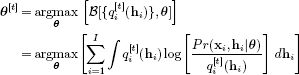
In the E-step at iteration t + 1, we set each distribution q_i(h_i) to be the posterior distributions Pr(h_i|x_i, θ) over that hidden variable given the associated data example and the current parameters θ^[t]. To compute these, we use Bayes’ rule

It can be shown that this choice maximizes the bound as much as possible.

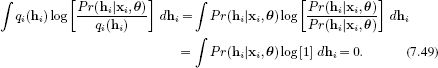
In the M-step, we directly maximize the bound (Equation 7.10) with respect to the parameters θ. In practice, we can simplify the expression for the bound to eliminate terms that do not depend on θ and this yields

Each of these steps is guaranteed to improve the bound, and iterating them alternately is guaranteed to find at least a local maximum with respect to θ.

This is a practical description of the EM algorithm, but there is a lot missing: we have not demonstrated that Equation 7.10 really is a bound on the log likelihood. We have not shown that the posterior distribution Pr(h_i|x_i, θ^[t]) is the optimal choice for q_i(h_i) in the E-step (Equation 7.11), and we have not demonstrated that the cost function for the M-step (Equation 7.2) improves the bound. For now we will assume that these things are true and proceed with the main thrust of the chapter. We will return to these issues in Section 7.8.

7.4 Mixture of Gaussians

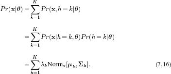
The mixture of Gaussians (MoG) is a prototypical example of a model where learning is suited to the EM algorithm. The data are described as a weighted sum of K normal distributions

where μ_1…K and Σ_1…K are the means and covariances of the normal distributions and λ_{1 … K} are positive valued weights that sum to one. The mixtures of Gaussians model describes complex multimodal probability densities by combining simpler constituent distributions (Figure 7.6).

To learn the parameters θ={μ_k, Σ_k, λ_k}^K_k=1 from training data {x_i}^I_i=1, we could apply the straightforward maximum likelihood approach

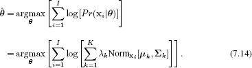
Unfortunately, if we take the derivative with respect to the parameters θ and equate the resulting expression to zero, it is not possible to solve the resulting equations in closed form. The sticking point is the summation inside the logarithm, which precludes a simple solution. Of course, we could use a nonlinear optimization approach, but this would be complex as we would have to maintain the constraints on the parameters: the weights λ must sum to one and the covariances {Σ_k}^K_k=1 must be positive definite. For a simpler approach, we express the observed density as a marginalization and use the EM algorithm to learn the parameters.

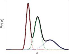
Figure 7.6 Mixture of Gaussians model in 1D. A complex multimodal probability density function (black solid curve) is created by taking a weighted sum or mixture of several constituent normal distributions with different means and variances (red, green, and blue dashed curves). To ensure that the final distribution is a valid density, the weights must be positive and sum to one.

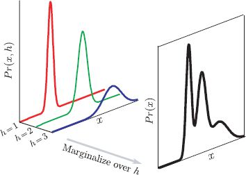
Figure 7.7 Mixture of Gaussians as a marginalization. The mixture of Gaussians can also be thought of in terms of a joint distribution Pr(x, h) between the observed variable x and a discrete hidden variable h. To create the mixture density, we marginalize over h. The hidden variable has a straightforward interpretation: it is the index of the constituent normal distribution.

7.4.1 Mixture of Gaussians as a marginalization

The mixture of Gaussians model can be expressed as the marginalization of a joint probability distribution between the observed data x and a discrete hidden variable h that takes values h ∈{1… K} (Figure 7.7). If we define

where λ = [λ₁… λ_K] are the parameters of the categorical distribution, then we can recover the original density using

Interpreting the model in this way also provides a method to draw samples from a mixture of Gaussians: we sample from the joint distribution Pr(x, h) and then discard the hidden variable h to leave just a data sample x. To sample from the joint distribution Pr(x, h), we first sample h from the categorical prior Pr(h), then sample x from the normal distribution Pr(x|h) associated with the value of h. Notice that the hidden variable h has a clear interpretation in this procedure. It determines which of the constituent normal distributions is responsible for the observed data point x.

7.4.2 Expectation maximization for fitting mixture models

To learn the MoG parameters θ ={λ_k, μ_k, Σ_k}^K_k=1 from training data {x_i}^I_i=1 we apply the EM algorithm. Following the recipe of Section 7.3, we initialize the parameters randomly and alternate between performing the E- and M-steps.

In the E-step, we maximize the bound with respect to the distributions q_i(h_i) by finding the posterior probability distribution Pr(h_i|x_i) of each hidden variable h_i given the observation x_i and the current parameter settings,

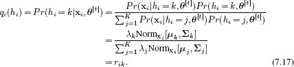
In other words we compute the probability Pr(h_i = k|x_i, θ^[t]) that the k^th normal distribution was responsible for the i^th datapoint (Figure 7.8). We denote this responsibility by r_ik for short.

In the M-step, we maximize the bound with respect to the model parameters θ = {λ_k, μ_k, Σ_k}^K_k=1 so that

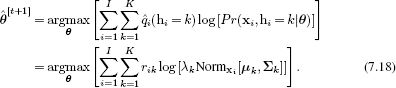
This maximization can be performed by taking the derivative of the expression with respect to the parameters, equating the result to zero, and rearranging, taking care to enforce the constraint Σ_k λ_k = 1 using Lagrange multipliers. The procedure results in the update rules:

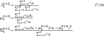
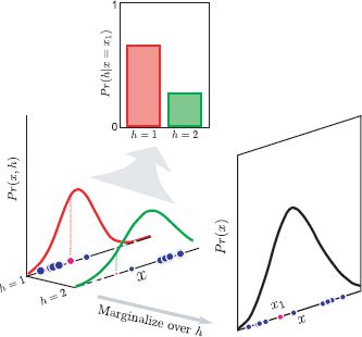
Figure 7.8 E-step for fitting the mixture of Gaussians model. For each of the I data points x_1…I, we calculate the posterior distribution Pr(h_i|x_i) over the hidden variable h_i. The posterior probability Pr(h_i = k|x_i) that h_i takes value k can be understood as the responsibility of normal distribution k for data point x_i. For example, for data point x₁ (magenta circle), component 1 (red curve) is more than twice as likely to be responsible than component 2 (green curve). Note that in the joint distribution (left), the size of the projected data point indicates the responsibility.

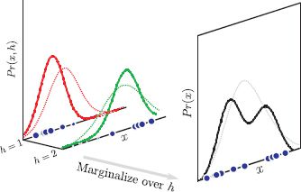
Figure 7.9 M-step for fitting the mixture of Gaussians model. For the k^th constituent Gaussian, we update the parameters {λ_k, μ_k, Σ_k}. The i^th data point x_i contributes to these updates according to the responsibility r_ik (indicated by size of point) assigned in the E-step; data points that are more associated with the k^th component have more effect on the parameters. Dashed and solid lines represent fit before and after the update, respectively.

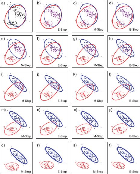
Figure 7.10 Fitting a mixture of two Gaussians to 2D data. a) Initial model. b) E-step. For each data point the posterior probability that is was generated from each Gaussian is calculated (indicated by color of point). c) M-step. The mean, variance and weight of each Gaussian is updated based on these posterior probabilities. Ellipse shows Mahalanobis distance of two. Weight (thickness) of ellipse indicates weight of Gaussian. d–t) Further E-step and M-step iterations.

These update rules can be easily understood (Figure 7.9): we update the weights {λ_k}^K_k=1 according to the relative total responsibility of each component for the data points. We update the cluster means {μ_k}^K_k=1 by computing the weighted mean over the datapoints where the weights are given by the responsibilities. If component k is mostly responsible for data point x_i, then this data point has a high weight and affects the update more. The update rule for the covariances has a similar interpretation.

In practice the E- and M-steps are alternated until the bound on the data no longer increases and the parameters no longer change. The alternating E-steps and M-steps for a two-dimensional example are shown in Figure 7.10. Notice that the final fit identifies the two clusters in the data. The mixture of Gaussians is closely related to clustering techniques such as the K-means algorithm (Section 13.4.4).

The EM approach to estimating mixture models has three attractive features.

1. Both steps of the algorithm can be computed in closed form without the need for an optimization procedure.

2. The solution guarantees that the constraints on the parameters are respected: the weighting parameters {λ_k}^K_k=1 are guaranteed to be positive and sum to one, and the covariance matrices {Σ_k}^K_k=1 are guaranteed to be positive definite.

3. The method can cope with missing data. Imagine that some of the elements of training example x_i are missing. In the E-step, the remaining dimensions can still be used to establish a distribution over the hidden variable h. In the M-step, this datapoint would contribute only to the dimensions of {μ_k}^K_k=1 and {Σ_k}^K_k=1 where data were observed.

Figure 7.11 shows a mixture of five Gaussians that has been fit to a 2D data set. As for the basic multivariate normal model, it is possible to constrain the covariance matrices to be spherical or diagonal. We can also constrain the covariances to be the same for each component if desired. Figure 7.12 shows the mean vectors μ_k for a ten-component model with diagonal covariances fitted to the face data set. The clusters represent different illumination conditions as well as changes in pose, expression, and background color.

In fitting mixtures of Gaussians, there are several things to consider. First, the EM algorithm does not guarantee to find a global solution to this non-convex optimization problem. Figure 7.13 shows three different solutions that were computed by starting the fitting algorithm with different initial random values for the parameters θ. The best we can do to circumvent this problem is to start fitting in different places and take the solution with the greatest log likelihood. Second, we must prespecify the number of mixing components. Unfortunately, we cannot decide the number of components by comparing the log likelihood: models with more parameters will inevitably describe the data better. There are methods to tackle this problem, but they are beyond the scope of this volume.

Finally, although we presented a maximum likelihood approach here, it is important in practice to include priors over model parameters Pr(θ) to prevent the scenario where one of the Gaussians becomes exclusively associated with a single datapoint. Without a prior, the variance of this component becomes progressively smaller and the likelihood increases without bound.

7.5 The t-distribution

The second significant problem with using the normal distribution to describe visual data is that it is not robust: the height of the normal pdf falls off very rapidly as we move into the tails. The effect of this is that outliers (unusually extreme observations) drastically affect the estimated parameters (Figure 7.14). The t-distribution is a closely related distribution in which the length of the tails is parameterized.

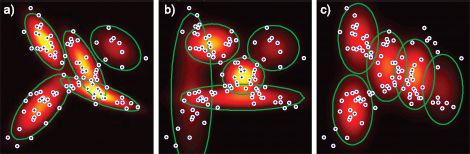
Figure 7.11 Covariance of components in mixture models. a) Full covariances. b) Diagonal covariances. c) Identical diagonal covariances.

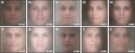
Figure 7.12 Mixtures of Gaussians model for face data. a–j) Mean vectors μ_k for a mixture of ten Gaussians fitted to the face data set. The model has captured variation in the mean luminance and chromaticity of the face and other factors such as the pose and background color. Numbers indicate the weight λ_kof each component.

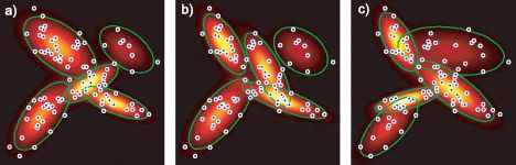
Figure 7.13 Local maxima. Repeated fitting of mixture of Gaussians model with different starting points results in different models as the fit converges to different local maxima. The log likelihoods are a) 98.76 b) 96.97 c) 94.35, respectively, indicating that (a) is the best fit.

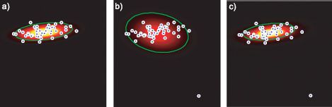
Figure 7.14 Motivation for t-distribution. a) The multivariate normal model fit to data. b) Adding a single outlier completely changes the fit. c) With the multivariate t-distribution the outlier does not have such a drastic effect.

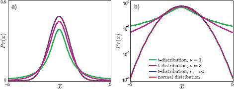
Figure 7.15 The univariate t-distribution. a) As well as the mean μ and scaling parameter σ², the t-distribution has a parameter ν which is termed the degrees of freedom. As ν decreases, the tails of the distribution become longer and the model becomes more robust. b) This is seen more clearly on a log scale.

The univariate t-distribution (Figure 7.15) has probability density function

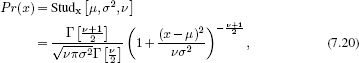
where μ is the mean and σ² is the scale parameter. The degrees of freedom ν ∈(0, ∞] controls the length of the tails: when ν is small there is considerable weight in the tails. For example, with μ = 0 and σ² = 1 a datapoint at x = −5 is roughly 10⁴ = 10000 times more likely under the t-distribution with ν = 1 than under the normal distribution. As ν tends to infinity, the distribution approximates a normal more and more closely and there is less weight in the tails. The variance of the distribution is given by σν/(ν − 2) for ν > 2 and infinite if 0 < ν ≤ 2.

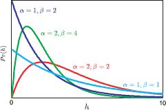
Figure 7.16 The gamma distribution is defined on positive real values and has two parameters α, β. The mean of the distribution is E[h] = α/β and the variance is E[(h − E[h])²] = α/β². The t-distribution can be thought of as a weighted sum of normal distributions with the same mean, but covariances that depend inversely on the gamma distribution.

The multivariate t-distribution has pdf

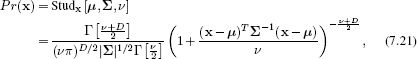
where D is the dimensionality of the space, μ is a D × 1 mean vector, Σ is a D × D positive definite scale matrix, and ν ∈ [0, ∞] is the degrees of freedom. As for the multivariate normal distribution (Figure 5.1), the scale matrix can take full, diagonal or spherical forms. The covariance of the distribution is given by Σν/(ν − 2) for ν > 2 and is infinite if 0 ≤ ν ≤ 2.

7.5.1 Student t-distribution as a marginalization

As for the mixtures of Gaussians, it is also possible to understand the t-distribution in terms of hidden variables. We define

where h is a scalar hidden variable and Gam[α, β] is the gamma distribution with parameters α, β (Figure 7.16). The gamma distribution is a continuous probability distribution defined on the positive real axis with probability density function

where Γ[•] is the gamma function.

The t-distribution is the marginalization with respect to the hidden variable h of the joint distribution between the data x and h (Figure 7.17),

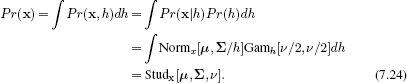
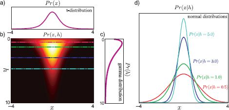
Figure 7.17 The t-distribution as a marginalization. a) The t-distribution has a similar form to the normal distribution but longer tails. b) The t-distribution is the marginalization of the joint distribution Pr(x, h) between the observed variable x and a hidden variable h. c) The prior distribution over the hidden variable h has a gamma distribution. d) The conditional distribution Pr(x|h) is normal with a variance that depends on h. So the t-distribution can be considered as an infinite weighted sum of normal distributions with variances determined by the gamma prior (equation 7.24).

This formulation also provides a method to generate data from the t-distribution. We first generate h from the gamma distribution and then generate x from the associated normal distribution Pr(x|h). Hence the hidden variable has a simple interpretation: it tells us which one of the continuous family of underlying normal distributions was responsible for this datapoint.

7.5.2 Expectation maximization for fitting t-distributions

Since the pdf takes the form of a marginalization of the joint distribution with a hidden variable (Equation 7.24), we can use the EM algorithm to learn the parameters θ = {μ, Σ, ν} from a set of training data {x_i}^I_i=1.

In the E-step (Figure 7.18a–b), we maximize the bound with respect to the distributions q_i(h_i) by finding the posterior Pr(h_i|x_i, θ^[t]) over each hidden variable h_i given associated observation x_i and the current parameter settings. By Bayes’ rule, we get

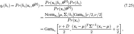
where we have used the fact that the gamma distribution is conjugate to the scaling factor for the normal variance. The E-step can be understood as follows: we are treating each data point x_i as if it were generated from one of the normals in the infinite mixture where the hidden variable h_i determines which normal. So, the E-step computes a distribution over h_i, which hence determines a distribution over which normal created the data.

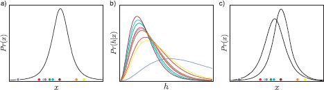
Figure 7.18 Expectation maximization for fitting t-distributions. a) Estimate of distribution before update. b) In the E-step, we calculate the posterior distribution Pr(h_i|x_i) over the hidden variable h_i for each data point x_i. The color of each curve corresponds to that of the original data point in (a). c) In the M-step, we use these distributions over h to update the estimate of the parameters θ = {μ, σ², ν}.

We now compute the following expectations (section 2.7) with respect to the distribution in Equation 7.25:

where Ψ[•]) is the digamma function. These expectations will be needed in the M-step.

In the M-step (Figure 7.18c) we maximize the bound with respect to the parameters θ = {μ, Σ, ν} so that

where the expectation is taken relative to the posterior distribution Pr(h_i|x_i, θ^[t]). Substituting in the expressions for the normal likelihood Pr(x_i|h_i) and the gamma prior Pr(h_i), we find that

To optimize μ and Σ, we take derivatives of Equation 7.28, set the resulting expressions to zero and rearrange to yield update equations

These update equations have an intuitive form: for the mean, we are computing a weighted sum of the data. Outliers in the data set will tend to be explained best by the normal distributions in the infinite mixture which have larger covariances: for these distributions h is small (h scales the normal covariance inversely). Consequently, E[h] is small, and they are weighted less in the sum. The update for the Σ has a similar interpretation.

Unfortunately, there is no closed form solution for the degrees of freedom ν. We hence perform a one-dimensional line search to maximize Equation 7.28 having substituted in the updated values of μ and Σ, or use one of the optimization techniques described in Chapter 9.

When we fit a t-distribution with a diagonal scale matrix Σ to the face data set, the mean μ and scale matrix Σ (not shown) look visually similar to those for the normal model (Figure 7.2). However, the model is not the same. The fitted degrees of freedom ν is 6.6. This low value indicates that the distribution has significantly longer tails than the normal model.

In conclusion, the multivariate t-distribution provides an improved description of data with outliers (Figure 7.14). It has just one more parameter than the normal (the degrees of freedom, ν), and subsumes the normal as a special case (where ν becomes very large). However, this generality comes at a cost: there is no closed form solution for the maximum likelihood parameters and so we must resort to more complex approaches such as the EM algorithm to fit the distribution.

7.6 Factor analysis

We now address the final problem with the normal distribution. Visual data are often very high dimensional: in the face detection task, the data comes in the form of 60 × 60 RGB images and is hence characterized as a 60 ×60 × 3 = 10800 dimensional vector. To model this data with the full multivariate normal distribution, we require a covariance matrix of dimensions 10800 × 10800: we would need a very large number of training examples to get good estimates of all of these parameters in the absence of prior information. Furthermore, to store the covariance matrix, we will need a large amount of memory, and there remains the problem of inverting this large matrix when we evaluate the normal likelihood (Equation 5.1).

Of course, we could just use the diagonal form of the covariance matrix, which contains only 10800 parameters. However, this is too great a simplification: we are assuming that each dimension of the data is independent and for face images this is clearly not true. For example, in the cheek region, the RGB values of neighboring pixels covary very closely. A good model should capture this information.

Factor analysis provides a compromise in which the covariance matrix is structured so that it contains fewer unknown parameters than the full matrix but more than the diagonal form. One way to think about the covariance of a factor analyzer is that it models part of the high-dimensional space with a full model and mops up remaining variation with a diagonal model.

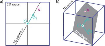
Figure 7.19 Linear subspaces. a) A one-dimensional subspace (a line through the origin, O) is embedded in a two-dimensional space. Any point x in the subspace can be reached by weighting the single basis vector ₁ appropriately. b) A two-dimensional subspace (a plane through the origin, O) is embedded in a three dimensional space. Any point x in the subspace can be reached using a linear combination x = α₁ + β₂ of the two basis functions ₁, ₂ that describe the subspace. In general, a K-dimensional subspace can be described using K basis functions.

More precisely, the factor analyzer describes a linear subspace with a full covariance model. A linear subspace is a subset of a high-dimensional space that can be reached by taking linear combinations (weighted sums) of a fixed set of basis functions (Figure 7.19). So, a line through the origin is a subspace in two dimensions as we can reach any point on it by weighting a single-basis vector. A line through the origin is also a subspace in three dimensions, but so is a plane through the origin: we can reach any point on the plane by taking linear combinations of two basis vectors. In general, a D-dimensional space contains subspaces of dimensions 1, 2, …, D − 1.

The probability density function of a factor analyzer is given by

where the covariance matrix ΦΦ^T + Σ contains a sum of two terms. The first term ΦΦ^T describes a full covariance model over the subspace: the K columns of the portrait¹ rectangular matrix Φ = [₁, ₂, …, _K] are termed factors. The factors are basis vectors that determine the subspace modeled. When we fit the model to data, the factors will span the set of directions where the data covary the most. The second term Σ is a diagonal matrix that accounts for all remaining variation.

Notice that this model has K × D parameters to describe Φ and another D parameters to describe the diagonal matrix Σ. If the number of factors K is much less than the dimensionality of the data D, then this model has fewer parameters than a normal with full covariance and hence can be learned from fewer training examples.

When Σ is a constant multiple of the identity matrix (i.e., models spherical covariance) the model is called probabilistic principal component analysis. This simpler model has slightly fewer parameters and can be fit in closed form (i.e., without the need for the EM algorithm), but otherwise it has no advantages over factor analysis (see Section 17.5.1 for more details). We will hence restrict ourselves to a discussion of the more general factor analysis model.

7.6.1 Factor analysis as a marginalization

As for the mixtures of Gaussians and the t-distribution, it is possible to view the factor analysis model as a marginalization of a joint distribution between the observed data x and a K-dimensional hidden variable h. We define

where I represents the identity matrix. It can be shown (but is not obvious) that

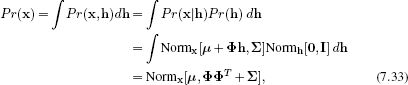
which was the original definition of the factor analyzer (Equation 7.31).

Expressing factor analysis as a marginalization reveals a simple method to draw samples from the distribution. We first draw a hidden variable h from the normal prior. We then draw the sample x from a normal distribution with mean μ + Φ h and diagonal covariance Σ (see Equation 7.32).

This leads us to a simple interpretation of the hidden variable h: each element h_k weights the associated basis function _k in the matrix Φ and so h defines a point on the subspace (Figure 7.19). The final density (Equation 7.31) is hence an infinite weighted sum of normal distributions with the same diagonal covariance Σ and means μ + Φ h that are distributed over the subspace. The relationship between mixture models and factor analysis is explored further in Figure 7.20.

7.6.2 Expectation maximization for learning factor analyzers

Since the factor analyzer can be expressed as a marginalization of a joint distribution between the observed data x and a hidden variable h (Equation 7.33), it is possible to use the EM algorithm to learn the parameters θ = {μ, Φ, Σ}. Once more, we follow the recipe described in Section 7.3.

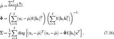
In the E-step (Figure 7.21), we optimize the bound with respect to the distributions q_i(h_i). To do this we compute the posterior probability distribution Pr(h_i|x_i) over each hidden variable h_i given the associated observed data x_i and the current values of the parameters θ^[t]. To this end we apply Bayes’ rule:

where we have made use of the change of variables relation (Section 5.7) and then the fact that the product of two normals is proportional to a third normal (Section 5.6). The resulting constant of proportionality exactly cancels out with the term Pr(x) in the denominator, ensuring that the result is a valid probability distribution.

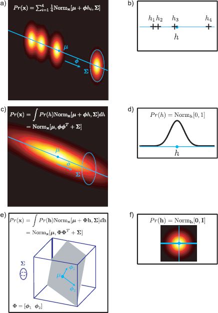
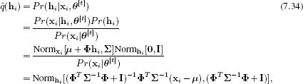
Figure 7.20 Relationship between factor analysis and mixtures of Gaussians. a) Consider an MoG model where each component has identical diagonal covariance Σ. We could describe variation in a particular direction by parameterizing the mean of each Gaussian as μ_i = μ + h_i. b) Different values of the scalar hidden variable h_i determine different positions along direction . c) Now we replace the MoG with an infinite sum (integral) over a continuous family of Gaussians, each of which is determined by a certain value of h. d) If we choose the prior over the hidden variable to be normal, this integral has a closed form solution and is a factor analyzer. e) More generally we want to describe variance in a set of directions Φ = [₁, ₂, …, _K] in a high dimensional space. f) To this end we use a K-dimensional hidden variable h and an associated normal prior Pr(h).

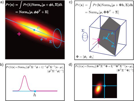
Figure 7.21 E-step for expectation maximization algorithm for factor analysis. a) Two-dimensional case with one factor. We are given a data point x (purple cross). b) In the E-step we seek a distribution over possible values of the associated hidden variable h. It can be shown that this posterior distribution over h is itself normally distributed. c) Three-dimensional case with two factors. Given a data point x (purple cross), we aim to find a distribution (d) over possible values of the associated hidden variable h. Once more this posterior is normally distributed.

The E-step computes a probability distribution over the possible causes h for the observed data. This implicitly defines a probability distribution over the positions Φ h on the subspace that might have generated this example.

We extract the following expectations from the posterior distribution (Equation 7.34) as they will be needed in the M-step:

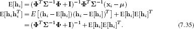
In the M-step, we optimize the bound with respect to the parameters θ= {μ, Φ, Σ} so that

where we have removed the term log[Pr(h_i) ] as it is not dependent on the variables θ. The expectations E[•] are taken with respect to the relevant posterior distributions _i(h_i) = Pr(h_i|x_i, θ^[t]). The expression for log[Pr(x_i|h_i)] is given by

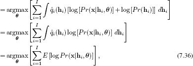
We optimize Equation 7.36 by taking derivatives with respect to the parameters θ = {μ, Φ, Σ}, equating the resulting expressions to zero and rearranging to yield

where the function diag[•] is the operation of setting all elements of the matrix argument to zero except those on the diagonal.

Figure 7.22 shows the parameters of a factor analysis model fitted to the face data using ten iterations of the EM algorithm. The different factors encode different modes of variation of the data set, which often have real-world interpretations such as changes in pose or lighting.

In conclusion, the factor analyzer is an efficient model for capturing the covariance in high-dimensional data. It devotes one set of parameters Φ to describing the directions in which the data are most correlated and a second set Σdescribes the remaining variation.

7.7 Combining models

The mixture of Gaussians, t-distribution, and factor analysis models are constructed similarly: each is a weighted sum or integral of a set of constituent normal distributions. Mixture of Gaussian models consist of a weighted sum of K normal distributions with different means and variances. The t-distribution consists of an infinite weighted sum of normal distributions with the same mean, but different covariances. Factor analysis models consist of an infinite weighted sum of normal distributions with different means, but the same diagonal covariance.

In light of these similarities, it is perhaps unsurprising then that the models can be easily combined. If we combine mixture models and factor analyzers, we get a mixture of factor analyzers (MoFA) model. This is a weighted sum of factor analyzers, each of which has a different mean and allocates high probability density to a different subspace. Similarly, combining mixture models and t-distributions results in a mixture of t-distributions or robust mixture model. Combining t-distributions and factor analyzers, we can construct a robust subspace model, which models data that lie primarily in a subspace but is tolerant to outliers. Finally, combining all three models, we get a mixture of robust subspace models. This has the combined benefits of all three approaches (it is multimodal and robust and makes efficient use of parameters). The associated density function is

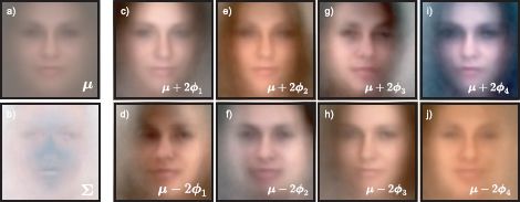
Figure 7.22 Factor analyzer with ten factors (four shown) for face classes. a) Mean μ for face model. b) Diagonal covariance component Σ for face model. To visualize the effect of the first factor ₁ we add (c) or subtract (d) a multiple of it from the mean: we are moving along one axis of the 10D subspace that seems to encode mainly the mean intensity. Other factors (e–j) encode changes in the hue and the pose of the face.

where μ_k, Φ_k and Σ_k represent the mean, factors and diagonal covariance matrix belonging to the k^th component, λ_k represents the weighting of the k^th component and ν_k represents the degrees of freedom of the k^th component. To learn this model, we would use a series of interleaved expectation maximization algorithms.

7.8 Expectation maximization in detail

Throughout this chapter, we have employed the expectation maximization algorithm, using the recipe from Section 7.3%. We now examine the EM algorithm in detail to understand why this recipe works.

The EM algorithm is used to find maximum likelihood or MAP estimates of model parameters θ where the likelihood Pr(x|θ) of the data x can be written as

and

for discrete and continuous hidden variables, respectively. In other words, the likelihood Pr(x|θ) is a marginalization of a joint distribution over the data and the hidden variables. We will work with the continuous case.

The EM algorithm relies on the idea of a lower bounding function (or lower bound), [θ] on the log likelihood. This is a function of the parameters θ that is always guaranteed to be equal to or lower than the log likelihood. The lower bound is carefully chosen so that it is easy to maximize with respect to the parameters.

This lower bound is also parameterized by a set of probability distributions {q_i(h_i)}^I_i=1 over the hidden variables, so we write it as [q_i(h_i)}, θ]. Different probability distributions q_i(h_i) predict different lower bounds [{q_i(h_i)}, θ] and hence different functions of θ that lie everywhere below the true log likelihood (Figure 7.5b).

In the EM algorithm, we alternate between expectation steps (E-steps) and maximization steps (M-steps) where

• in the E-step (Figure 7.23a) we fix θ and find the best lower bound [{q_i(h_i)}, θ] with respect to the distributions q_i(h_i). In other words, at iteration t

The best lower bound will be a function that is as high as possible at the current parameter estimates θ. Since it must be everywhere equal to or lower than the log likelihood, the highest possible value is the log likelihood itself. So the bound touches the log-likelihood curve for the current parameters θ.

• in the M-step (Figure 7.23b), we fix q_i(h_i) and find the values of θ that maximize this bounding function [{q_i(h_i)}, θ]. In other words, we compute

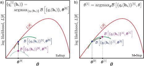
Figure 7.23 E-step and M-step. a) In the E-step, we manipulate the distributions {q_i(h_i)} to find the best new lower bound given parameters θ. This optimal lower bound will touch the log likelihood at the current parameter values θ (we cannot do better than this!). b) In the M-step, we hold {q_i(h_i)} constant and optimize θ with respect to the new bound.

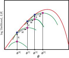
Figure 7.24 Expectation maximization algorithm. We iterate the expectation and maximization steps by alternately changing the distributions q_i(h_i) and the parameter θ so that the bound increases. In the E-step, the bound is maximized with respect to q_i(h_i) for fixed parameters θ: the new function with respect to θ touches the true log likelihood at θ. In the M-step, we find the maximum of this function. In this way we are guaranteed to reach a local maximum in the likelihood function.

By iterating these steps, the (local) maximum of the actual log likelihood is approached (Figure 7.24). To complete our picture of the EM algorithm, we must

• Define [{q_i(h_i)}, θ^[t−1]] and show that it always lies below the log likelihood,

• Show which probability distribution q_i(h_i) optimizes the bound in the E-step,

• Show how to optimize the bound with respect to θ in the M-step.

These three issues are tackled in Sections 7.8.1, 7.8.2 and 7.8.3, respectively.

7.8.1 Lower bound for EM algorithm

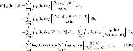
We define the lower bound [{q_i(h_i)}, θ] to be

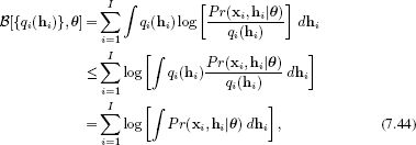
where we have used Jensen’s inequality between the first and second lines. This states that because the logarithm is a concave function, we can write

or E[log[y]] ≤ log(E[y]). Figure 7.25 illustrates Jensen’s inequality for a discrete variable.

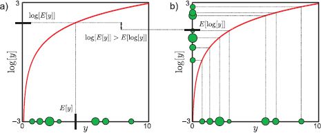
Figure 7.25 Jensen’s inequality for the logarithmic function (discrete case). a) Taking a weighted average of examples E[y] and passing them through the log function. b) Passing the samples through the log function and taking a weighted average E[log[y]]. The latter case always produces a smaller value than the former (E[log[y]] ≤ log(E[y]) ≤ log(E[y])): higher valued examples are relatively compressed by the concave log function.

7.8.2 The E-Step

In the E-step, we update the bound [q_i(h_i)}, θ] with respect to the distributions q_i(h_i). To see how to do this, we manipulate the expression for the bound as follows:

where the hidden variables from the first term are integrated out between the last two lines. The first term in this expression is constant with respect to the distributions q_i(h_i), and so to optimize the bound we must find the distributions _i(h_i) that satisfy

This expression is known as the Kullback-Leibler divergence q_i(h_i) and Pr(h_i|x_i, θ). It is a measure of distance between probability distributions. We can use the inequality log[y] ≤ y − 1 (plot the functions to convince yourself of this!) to show that this cost function (including the minus sign) is always positive,

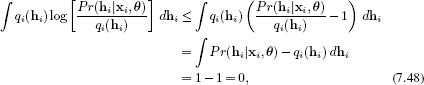
implying that when we reintroduce the minus sign the cost function must be positive. So the criteria in Equation 7.46 will be maximized when the Kullback-Leibler divergence is zero. This value is reached when q_i(h_i) = Pr(h_i|x_i, θ) so that

In other words, to maximize the bound with respect to q_i(h_i), we set this to be the posterior distribution Pr(h_i|x_i, θ) over the hidden variables h_i given the current set of parameters. In practice, this is computed using Bayes’ rule,

So the E-step consists of computing the posterior distribution for each hidden variable using Bayes’ rule.

7.8.3 The M-Step

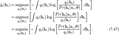
In the M-step, we maximize the bound with respect to the parameters θ so that

where we have omitted the second term as it does not depend on the parameters. If you look back at the algorithms in this chapter, you will see that we have maximized exactly this criterion.

7.9 Applications

The models in this chapter have many uses in computer vision. We now present a cross-section of applications. As an example of two-class classification using mixtures of Gaussians densities, we reconsider the face detection application that has been a running theme throughout this chapter. To illustrate multiclass classification, we describe an object recognition model based on t-distributions. We also describe a segmentation application which is an example of unsupervised learning: we do not have labeled training data to build our model.

To illustrate the use of the factor analyzer for classification, we present a face recognition example. To illustrate its use for regression, we consider the problem of changing a face image from one pose to another. Finally, we highlight the fact that hidden variables can take on real-world interpretations by considering a model that explains the weak spatial alignment of digits.

7.9.1 Face detection

In face detection, we attempt to infer a discrete label w ∈ {0, 1} indicating whether a face is present or not based on observed data x. We will describe the likelihood for each world state with a mixtures of Gaussians model, where the covariances of the Gaussian components are constrained to be diagonal so that

where m indexes the world state and k indexes the component of the mixture distribution.

We will assume that we have no prior knowledge about whether the face is present or not so that Pr(w = 0) = Pr(w = 1) = 0.5. We fit the two likelihood terms using a set of labeled training pairs {x_i, w_i}. In practice this means learning one mixtures of Gaussians model for the non-faces based on the data where w_i = 0 and a separate model for the faces based on the data where w = 1.

For test data x*, we compute the posterior probability over w using Bayes’ rule:

Table 7.1 shows percent correct classification for 100 test examples The results are based on models learned from 1000 training examples of each class.

Table 7.1 Percent correct classification rates for two different models and three different types of preprocessing. In each case, the data x* was assigned to be a face if the posterior probability Pr(w = 1|x*) was greater than 0.5.

The first column shows results where the data vector consists of the RGB values with a 24 × 24 region (the running example in this chapter used 60 × 60 pixel regions, but this is unnecessarily large). The results are compared to classification based on a single normal distribution. The subsequent columns of the table show results for systems trained and tested with grayscale 24 × 24 pixel regions and grayscale 24 × 24 regions that have been histogram equalized (Section 13.1.2).

There are two insights to be gleaned from these classification results. First, the choice of model does make a difference: the mixtures of Gaussians density always results in better classification performance than the single Gaussian model. Second, the choice of preprocessing is also critical to the final performance. This book concerns models for vision, but it is important to understand that this is not the only thing that determines the final performance of real-world systems. A brief summary of preprocessing methods is presented in Chapter 13.

The reader should not depart with the impression that this is a sensible approach to face detection. Even the best performance of 89% is far below what would be required in a real face detector: consider that in a single image we might classify patches at 10000 different positions and scales, so an 11% error rate will be unacceptable. Moreover, evaluating each patch under both class conditional density functions is too computationally expensive to be practical. In practice, face detection would normally be achieved using discriminative methods (see Chapter 9).

7.9.2 Object recognition

In object recognition, the goal is to assign a discrete world vector w_i ∈{1, 2, …, M} indicating which of M categories is present based on observed data x_i from the i^th image. To this end, Aeschliman et al. 2010 split each image into 100 10 × 10 pixel regions arranged in a regular grid. The grayscale pixel data x_ij from the j^th region of the i^th image were concatenated to form a 100 × 1 vector x_ij. They treated the regions independently and described each with a t-distribution so that the class conditional density functions were

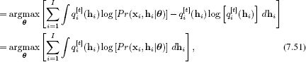
Figure 7.26 shows results based on training with 10 classes from the Amsterdam library of images (Geusebroek et al. 2005). Each class consists of 72 images taken at 5-degree intervals around the object. The data were divided randomly into 36 test images and 36 training images for each class. The prior probabilities of the classes were set to uniform, and the posterior distribution Pr(w_i|x_i) was calculated using Bayes’ rule. A test object was classified according to the class with the highest posterior probability.

Figure 7.26 Object recognition. a) The training database consists of a series of different views of ten different objects. The goal is to learn a class-conditional density function for each object and classify new examples using Bayes’ rule. b) Percent correct results for class conditional densities based on the t-distribution (top row) and the normal distributions (bottom row). The robust model performs better, especially on objects with specularities. Images from Amsterdam library (Guesebroek et al. 2005).

The results show the superiority of the t-distribution – for almost every class; the percent correct performance is better, and this is especially true for objects such as the china pig where the specularities act as outliers. By adding just one more parameter per patch, the performance increases from a mean of 51% to 68%.

7.9.3 Segmentation

The goal of segmentation is to assign a discrete label {w_n}^N_n=1 which takes one of K values w_n ∈ {1,2,…, K} to each of the N pixels in the image so that regions that belong to the same object are assigned the same label. The segmentation model depends on observed data vectors {x_n}^N_n=1 at each of the N pixels that would typically include the (x, y) position of the pixel and other information characterizing local texture.

We will frame this problem as unsupervised learning. In other words, we do not have the luxury of having training images where the state of the world is known. We must both learn the parameters θ and estimate the world states {w_i}^I_i=1 from the image data {x_n}^N_n=1.

We will assume that the k^th object is associated with a normal distribution with parameters μ_k and ∑_k and prevalence λ_k so that

Marginalizing out the world state w, we have

To fit this model, we find the parameters θ = {λ_k, μ_k, Σ_k}^K_k=1 using the EM algorithm. To assign a class to each pixel, we then find the value of the world state that has the highest posterior probability given the observed data

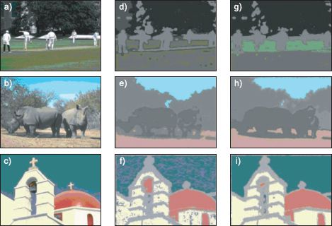
Figure 7.27 Segmentation. a–c) Original images. d–f) Segmentation results based on a mixture of five normal distributions. The pixels associated with the k^th component are colored with the mean RGB values of the pixels that are assigned to this value. g–i) Segmentation results based on a mixture of K t-distributions. The segmentation here is less noisy than for the MoG model. Results from Sfikas et al. (2007). © IEEE 2007.

where the posterior is computed as in the E-step.

Figure 7.27 shows results from this model and a similar mixture model based on t-distributions from Sfikas et al. (2007). The mixture models manage to partition the image quite well into different regions. Unsurprisingly, the t-distribution results are rather less noisy than those based on the normal distribution.

7.9.4 Frontal face recognition

The goal of face identification (Figure 7.28 is to assign a label w ∈ {1… M} indicating which of M possible identities the face belongs to based on a data vector x. The model is learned from labeled training data {x_i, w_i}^I_i=1 where the identity is known. In a simple system, the data vector might consist of the concatenated grayscale values from the face image, which should be reasonably large (say 50 ×50 pixels) to ensure that the identity is well represented.

Since the data are high-dimensional, a reasonable approach is to model each class conditional density function with a factor analyzer

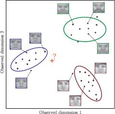
Figure 7.28 Face recognition. Our goal is to take the RGB values of a facial image x and assign a label w ∈ {1… K} corresponding to the identity. Since the data are high-dimensional, we model the class conditional density function Pr(x|w = k) for each individual in the database as a factor analyzer. To classify a new face, we apply Bayes’ rule with suitable priors Pr(w) to compute the posterior distribution Pr(w|x). We choose the label = argmax_w [Pr(w = k|x)] that maximizes the posterior. This approach assumes that there are sufficient training examples to learn a factor analyzer for each class.

where the parameters for the k^th identity θ_k = μ_k, Φ_k, ∑_k can be learned from the subset of data that belongs to that identity using the EM algorithm. We also assign priors P(w = k) according to the prevalence of each identity in the database.

To perform recognition, we compute the posterior distribution Pr(w*|x*) for the new data example x* using Bayes’ rule. We assign the identity that maximizes this posterior distribution.

This approach works well if there are sufficient examples of each gallery individual to learn a factor analyzer, and if the poses of all of the faces are similar. In the next example, we develop a method to change the pose of faces, so that we can cope when the poses of the faces differ.

7.9.5 Changing face pose (regression)

To change the pose of the face, we predict the RGB values w of the face in the new pose given a face x in the old pose. This is different from the previous examples in that it is a regression problem: the output w is a continuous multidimensional variable rather than a class label.

We form a compound variable z = [x^T w^T]^T by concatenating the RGB values from the two poses together. We now model the joint density as Pr(z) = Pr(x, w) with a factor analyzer

which we learn for paired training examples {x_i, w_i}^I_i=1 where the identity is known to be the same for each pair.

To find the non-frontal face w* corresponding to a new frontal face x* we use the approach of Section 6.3.2: the posterior over w* is just the conditional distribution Pr(w|x). Since the joint distribution is normal, we can compute the posterior distribution in closed form using equation 5.5. Using the notation

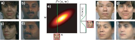
Figure 7.29 Regression example: we aim to predict quarter-left face image w from the frontal image x. To this end, we take paired examples of frontal faces (a–b) and quarter-left faces (c–d) and learn a joint probability model Pr(x, w) by concatenating the variables to form z = [x^T, w^T]^T and fitting a factor analyzer to z. e) Since the factor analyzer has a normal density (Equation 7.31), we can predict the conditional distribution Pr(w|x) of a quarter-left face given a frontal face which will also be normal (see section 5.5). f–g) Two frontal faces. h–i) MAP predictions for non-frontal faces (the mean of the normal distribution Pr(w|x)).

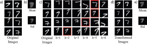
Figure 7.30 Modeling transformations with hidden variables. a) The original set of digit images are only weakly aligned. b) The mean and standard deviation images are consequently blurred out. The probability density model does not fit well. c) Each possible value of a discrete hidden variable represents a different transformation (here inverse transformations are shown). The red square highlights the most likely choice of hidden variable after ten iterations. d) The inversely transformed digits (based on most likely hidden variable). d) The new mean and standard deviation images are more focused: the probability density function fits better.

the posterior is given by

and the most probable w* is at the mean of this distribution.

7.9.6 Transformations as hidden variables

Finally, we consider a model that is closely related to the mixture of Gaussians, but where the hidden variables have a clear real-world interpretation. Consider the problem of building a density function for a set of poorly aligned images of digits (Figure 7.30). A simple normal distribution with diagonal covariance produces only a very poor representation of the data because most of the variation is due to the poor alignment.

We construct a generative model that first draws an aligned image x′ from a normal distribution, and then translates it using one of a discrete set {trans_k[•]}^K_k=1 of K possible transformations to explain the poorly aligned image x. In mathematical terms, we have

where h ∈{1,…, K} is a hidden variable that denotes which of the possible transformations warped this example.

This model can be learned using an EM-like procedure. In the E-step, we compute a probability distribution Pr(h_i|x_i) over the hidden variables by applying all of the inverse transformations to the each example and evaluating how likely the result is under the current parameters μ and Σ. In the M-step, we update these parameters by taking weighted sums of the inverse transformed images.

Summary

In this chapter we have introduced the idea of the hidden variable to induce structure in density models. The main approach to learning models of this kind is the expectation maximization algorithm. This is an iterative approach that is only guaranteed to find a local maximum. We have seen that although these models are more sophisticated than the normal distribution, they are still not really good representations of the density of high-dimensional visual data.

Notes

Expectation maximization: The EM algorithm was originally described by Dempster et al. (1977) although the presentation in this chapter owes more to the perspective espoused in Neal and Hinton (1999). A comprehensive summary of the EM algorithm and its extensions can be found in McLachlan and Krishnan (2008).

Mixtures of Gaussians: The mixtures of Gaussians model is closely related to the K-means algorithm (discussed in Section 13.4.4), which is a pure clustering algorithm, but does not have a probabilistic interpretation. Mixture models are used extensively in computer vision. Common applications include skin detection (e.g., Jones and Rehg 2002) and background subtraction (e.g., Stauffer and Grimson 1999).

t-distribution: General information about the t-distribution can be found in kotz and Nadarajah (2004). The EM algorithm for fitting the t-distribution is given in Liu and Rubin (1995), and other fitting methods are discussed in Nadarajh and Kotz (2008) and Aeschliman et al. (2010). Applications of t-distributions in vision include object recognition Aeschliman et al. (2010) and tracking Loxam and Drummond 2008, Aeschliman et al. 2010), and they are also used as the building blocks of sparse image priors (Roth and Black 2009).

Subspace models: The EM algorithm to learn the factor analyzer is due to Rubin and Thayer (1982). Factor analysis is closely related to several other models including probabilistic principal component analysis Tipping and Bishop (1999), which is discussed in Section 17.5.1, and principal component analysis, which is discussed in Section 13.4.2. Subspace models have been extended to the nonlinear case by Lawrence (2004). This is discussed in detail in Section 17.8. In Chapter 18, we present a series of models based on factor analysis which explicitly encode the identity and style of the object.

Combining models: Ghahramani and Hinton (1996c) introduced the mixtures of factor analyzers model. Peel and McLachlan (2000) present an algorithm for learning robust mixture models Mixtures of t-distributions).Khan and Dellaert (2004) and Zhao and Jiang (2006) both present subspace models based on the t-distribution. De Ridder and Franc (2003) combined mixture models, subspace models and t-distributions to create a distribution that is mutli-modal, robust and oriented along a subspace.

Face detection, face recognition, object recognition: Models based on subspace distributions were used in early methods for face and object recognition (e.g., Moghaddam and Pentland 1997, Murase and Nayar 1995). Modern face detection methods mainly rely on discriminative methods (Chapter 9), and the current state of the art in object recognition relies on bag of words approaches (chapter 20). Face recognition applications do not usually have the luxury of having many examples of each individual and so cannot build a separate density for each. However, modern approaches are still largely based on subspace methods (see Chapter 18).

Segmentation: Belongie et al. (1998) use a mixtures of Gaussians scheme similar to that described to segment the image as part of a content-based image retrieval system. A modern approach to segmentation based on the mixture of Gaussians model can be found in Ma et al. (2007). Sfikas et al. (2007) compared the segmentation performance of mixtures of Gaussians and mixtures of t-distributions.

Other uses for hidden variables: Frey and Jojic (1999a), (1999b) used hidden variables to model unseen transformations applied to data from mixture models and subspace models, respectively. Jojic and Frey (2001) used discrete hidden variables to represent the index of the layer in a multilayered model of a video. Jojic et al. (2003) presented a structured mixture model, where the mean and variance parameters are represented as an image and the hidden variable indexes the starting position of subpatch from this image.

Problems

7.1 Consider a computer vision system for machine inspection of oranges in which the goal is to tell if the orange is ripe. For each image we separate the orange from the background and calculate the average color of the pixels, which we describe as a 3 × 1 vector x. We are given training pairs {x_i, w_i} of these vectors, each with an associated binary variable w ∈ {0, 1} that indicates that this training example was unripe (w = 0) or ripe (w = 1). Describe how to build a generative classifier that could classify new examples x* as being ripe or unripe.

7.2 It turns out that a small subset of the training labels w_i in the previous example were wrong. How could you modify your classifier to cope with this situation?

7.3 Derive the M-step equations for the mixtures of Gaussians model (Equation 7.19).

7.4 Consider modeling some univariate continuous visual data x ∈[0,1] using a mixture of beta distributions. Write down an equation for this model. Describe in words what will occur in (i) the E-step and (ii) the M-step.

7.5 Prove that the student t-distribution over x is the marginalization with respect to h of the joint distribution Pr(x, h) between x and a hidden variable h where

7.6 Show that the peak of the Gamma distribution Gam_z[α, β] is at

7.7 Show that the Gamma distribution is conjugate to the inverse scaling factor of the variance in a normal distribution so that

and find the constant of proportionality and the new parameters α and β.

7.8 The model for factor analysis can be written as

where h_i is distributed normally with mean zero and identity covariance and ∈_i is distributed normally with mean zero and covariance ∑. Determine expressions for

1. E[x_i],

2. E[(x_i − E[x_i])²].

7.9 Derive the E-step for factor analysis (Equation 7.34).

7.10 Derive the M-step for factor analysis (Equation 7.38).

___________________________________

¹That is, it is tall and thin as opposed to landscape, which would be short and wide.