Introduction to 3D Game Programming with DirectX 12 (Computer Science) (2016)

Part 2

DIRECT3D
FOUNDATIONS

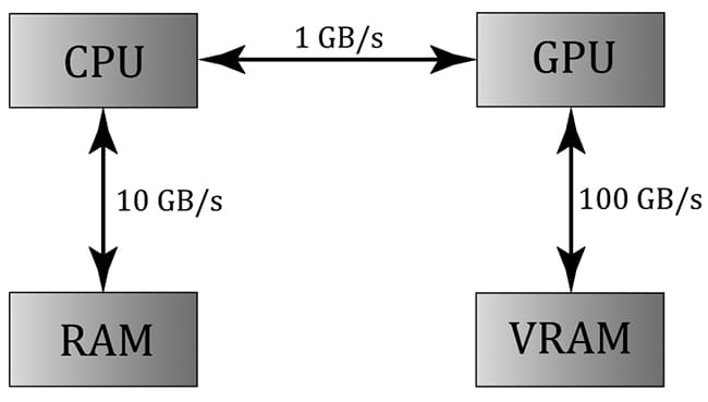
GPUs have been optimized to process a large amount of memory from a single location or sequential locations (so-called streaming operation); this is in contrast to a CPU designed for random memory accesses [Boyd10]. Moreover, because vertices and pixels can be independently processed, GPUs have been architected to be massively parallel; for example, the NVIDIA “Fermi” architecture supports up to sixteen streaming multiprocessors of thirty-two CUDA cores for a total of 512 CUDA cores [NVIDIA09].

Obviously, graphics benefit from this GPU architecture, as the architecture was designed for graphics. However, some non-graphical applications benefit from the massive amount of computational power a GPU can provide with its parallel architecture. Using the GPU for non-graphical applications is called general purpose GPU (GPGPU) programming. Not all algorithms are ideal for a GPU implementation; GPUs need data-parallel algorithms to take advantage of the parallel architecture of the GPU. That is, we need a large amount of data elements that will have similar operations performed on them so that the elements can be processed in parallel. Graphical operations like shading pixels is a good example, as each pixel fragment being drawn is operated on by the pixel shader. As another example, if you look at the code for our wave simulation from the previous chapters, you will see that in the update step, we perform a calculation on each grid element. So this, too, is a good candidate for a GPU implementation, as each grid element can be updated in parallel by the GPU. Particle systems provide yet another example, where the physics of each particle can be computed independently provided we take the simplification that the particles do not interact with each other.

For GPGPU programming, the user generally needs to access the computation results back on the CPU. This requires copying the result from video memory to system memory, which is slow (see Figure 13.1), but may be a negligible issue compared to the speed up from doing the computation on the GPU. For graphics, we typically use the computation result as an input to the rendering pipeline, so no transfer from GPU to CPU is needed. For example, we can blur a texture with the compute shader, and then bind a shader resource view to that blurred texture to a shader as input.

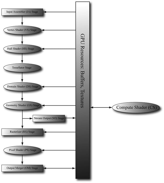
Figure 13.1. Image has been redrawn from [Boyd10]. The relative memory bandwidth speeds between CPU and RAM, CPU and GPU, and GPU and VRAM. These numbers are just illustrative numbers to show the order of magnitude difference between the bandwidths. Observe that transferring memory between CPU and GPU is the bottleneck.

The Compute Shader is a programmable shader Direct3D exposes that is not directly part of the rendering pipeline. Instead, it sits off to the side and can read from GPU resources and write to GPU resources (Figure 13.2). Essentially, the Compute Shader allows us to access the GPU to implement data-parallel algorithms without drawing anything. As mentioned, this is useful for GPGPU programming, but there are still many graphical effects that can be implemented on the compute shader as well—so it is still very relevant for a graphics programmer. And as already mentioned, because the Compute Shader is part of Direct3D, it reads from and writes to Direct3D resources, which enables us to bind the output of a compute shader directly to the rendering pipeline.

Figure 13.2. The compute shader is not part of the rendering pipeline but sits off to the side. The compute shader can read and write to GPU resources. The compute shader can be mixed with graphics rendering, or used alone for GPGPU programming.

Objectives:

1. To learn how to program compute shaders.

2. To obtain a basic high-level understanding of how the hardware processes thread groups, and the threads within them.

3. To discover which Direct3D resources can be set as an input to a compute shader and which Direct3D resources can be set as an output to a compute shader.

4. To understand the various thread IDs and their uses.

5. To learn about shared memory and how it can be used for performance optimizations.

6. To find out where to obtain more detailed information about GPGPU programming.

13.1 THREADS AND THREAD GROUPS

In GPU programming, the number of threads desired for execution is divided up into a grid of thread groups. A thread group is executed on a single multiprocessor. Therefore, if you had a GPU with sixteen multiprocessors, you would want to break up your problem into at least sixteen thread groups so that each multiprocessor has work to do. For better performance, you would want at least two thread groups per multiprocessor since a multiprocessor can switch to processing the threads in a different group to hide stalls [Fung10] (a stall can occur, for example, if a shader needs to wait for a texture operation result before it can continue to the next instruction).

Each thread group gets shared memory that all threads in that group can access; a thread cannot access shared memory in a different thread group. Thread synchronization operations can take place amongst the threads in a thread group, but different thread groups cannot be synchronized. In fact, we have no control over the order in which different thread groups are processed. This makes sense as the thread groups can be executed on different multiprocessors.

A thread group consists of n threads. The hardware actually divides these threads up into warps (thirty-two threads per warp), and a warp is processed by the multiprocessor in SIMD32 (i.e., the same instructions are executed for the thirty-two threads simultaneously). Each CUDA core processes a thread and recall that a “Fermi” multiprocessor has thirty-two CUDA cores (so a CUDA core is like an SIMD “lane.”) In Direct3D, you can specify a thread group size with dimensions that are not multiples of thirty-two, but for performance reasons, the thread group dimensions should always be multiples of the warp size [Fung10].

Thread group sizes of 256 seems to be a good starting point that should work well for various hardware. Then experiment with other sizes. Changing the number of threads per group will change the number of groups dispatched.

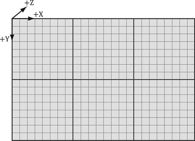
In Direct3D, thread groups are launched via the following method call:

void ID3D12GraphicsCommandList::Dispatch(

UINT ThreadGroupCountX,

UINT ThreadGroupCountY,

UINT ThreadGroupCountZ);

This enables you to launch a 3D grid of thread groups; however, in this book we will only be concerned with 2D grids of thread groups. The following example call launches three groups in the x direction and two groups in the y direction for a total of 3 × 2 = 6 thread groups (see Figure 13.3).

Figure 13.3. Dispatching a grid of 3 × 2 thread groups. Each thread group has 8 × 8 threads.

13.2 A SIMPLE COMPUTE SHADER

Below is a simple compute shader that sums two textures, assuming all the textures are the same size. This shader is not very interesting, but it illustrates the basic syntax of writing a compute shader.

cbuffer cbSettings

{

// Compute shader can access values in constant buffers.

};

// Data sources and outputs.

Texture2D gInputA;

Texture2D gInputB;

RWTexture2D<float4> gOutput;

// The number of threads in the thread group. The threads in a group can

// be arranged in a 1D, 2D, or 3D grid layout.

[numthreads(16, 16, 1)]

void CS(int3 dispatchThreadID : SV_DispatchThreadID) // Thread ID

{

// Sum the xyth texels and store the result in the xyth texel of

// gOutput.

gOutput[dispatchThreadID.xy] =

gInputA[dispatchThreadID.xy] +

gInputB[dispatchThreadID.xy];

}

A compute shader consists of the following components:

1. Global variable access via constant buffers.

2. Input and output resources, which are discussed in the next section.

3. The [numthreads(X, Y, Z)] attribute, which specifies the number of threads in the thread group as a 3D grid of threads.

4. The shader body that has the instructions to execute for each thread.

5. Thread identification system value parameters (discussed in §13.4).

Observe that we can define different topologies of the thread group; for example, a thread group could be a single line of X threads [numthreads(X, 1, 1)] or a single column of Y threads [numthreads(1, Y, 1)]. 2D thread groups of X × Y threads can be made by setting the z-dimension to 1 like this [numthreads(X, Y, 1)]. The topology you choose will be dictated by the problem you are working on. As mentioned in the previous section, the total thread count per group should be a multiple of the warp size (thirty-two for NVIDIA cards) or a multiple of the wavefront size (sixty-four for ATI cards). A multiple of the wavefront size is also a multiple of the warp size, so choosing a multiple of the wavefront size works for both types of cards.

13.2.1 Compute PSO

To enable a compute shader, we use a special “compute pipeline state description.” This structure has far fewer fields than D3D12_GRAPHICS_PIPELINE_STATE_DESC because the compute shader sits to the side of the graphics pipeline, so all the graphics pipeline state does not apply to compute shaders and thus does not need to be set. Below shows an example of creating a compute pipeline state object:

D3D12_COMPUTE_PIPELINE_STATE_DESC wavesUpdatePSO = {};

wavesUpdatePSO.pRootSignature = mWavesRootSignature.Get();

wavesUpdatePSO.CS =

{

reinterpret_cast<BYTE*>(mShaders["wavesUpdateCS"]->GetBufferPointer()),

mShaders["wavesUpdateCS"]->GetBufferSize()

};

wavesUpdatePSO.Flags = D3D12_PIPELINE_STATE_FLAG_NONE;

ThrowIfFailed(md3dDevice->CreateComputePipelineState(

&wavesUpdatePSO, IID_PPV_ARGS(&mPSOs["wavesUpdate"])));

The root signature defines what parameters the shader expects as input (CBVs, SRVs, etc.). The CS field is where we specify the compute shader. The following code shows an example of compiling a compute shader to bytecode:

mShaders["wavesUpdateCS"] = d3dUtil::CompileShader(

L"Shaders\\WaveSim.hlsl", nullptr, "UpdateWavesCS", "cs_5_0");

13.3 DATA INPUT AND OUTPUT RESOURCES

Two types of resources can be bound to a compute shader: buffers and textures. We have worked with buffers already such as vertex and index buffers, and constant buffers. We are also familiar with texture resources from Chapter 9.

13.3.1 Texture Inputs

The compute shader defined in the previous section defined two input texture resources:

Texture2D gInputA;

Texture2D gInputB;

The input textures gInputA and gInputB are bound as inputs to the shader by creating (SRVs) to the textures and passing them as arguments to the root parameters; for example:

cmdList->SetComputeRootDescriptorTable(1, mSrvA);

cmdList->SetComputeRootDescriptorTable(2, mSrvB);

This is exactly the same way we bind shader resource views to pixel shaders. Note that SRVs are read-only.

13.3.2 Texture Outputs and Unordered Access Views (UAVs)

The compute shader defined in the previous section defined one output resource:

RWTexture2D<float4> gOutput;

Outputs are treated special and have the special prefix to their type “RW,” which stands for read-write, and as the name implies, you can read and write to elements in this resource in the compute shader. In contrast, the textures gInputA and gInputB are read-only. Also, it is necessary to specify the type and dimensions of the output with the template angle brackets syntax <float4>. If our output was a 2D integer like DXGI_FORMAT_R8G8_SINT, then we would have instead written:

RWTexture2D<int2> gOutput;

Binding an output resource is different than an input, however. To bind a resource that we will write to in a compute shader, we need to bind it using a new view type called an unordered access view (UAV), which is represented in code by a descriptor handle and described in code by the D3D12_UNORDERED_ACCESS_VIEW_DESC structure. This is created in a similar way to a shader resource view. Here is an example that creates a UAV to a texture resource:

D3D12_RESOURCE_DESC texDesc;

ZeroMemory(&texDesc, sizeof(D3D12_RESOURCE_DESC));

texDesc.Dimension = D3D12_RESOURCE_DIMENSION_TEXTURE2D;

texDesc.Alignment = 0;

texDesc.Width = mWidth;

texDesc.Height = mHeight;

texDesc.DepthOrArraySize = 1;

texDesc.MipLevels = 1;

texDesc.Format = DXGI_FORMAT_R8G8B8A8_UNORM;

texDesc.SampleDesc.Count = 1;

texDesc.SampleDesc.Quality = 0;

texDesc.Layout = D3D12_TEXTURE_LAYOUT_UNKNOWN;

texDesc.Flags = D3D12_RESOURCE_FLAG_ALLOW_UNORDERED_ACCESS;

ThrowIfFailed(md3dDevice->CreateCommittedResource(

&CD3DX12_HEAP_PROPERTIES(D3D12_HEAP_TYPE_DEFAULT),

D3D12_HEAP_FLAG_NONE,

&texDesc,

D3D12_RESOURCE_STATE_COMMON,

nullptr,

IID_PPV_ARGS(&mBlurMap0)));

D3D12_SHADER_RESOURCE_VIEW_DESC srvDesc = {};

srvDesc.Shader4ComponentMapping = D3D12_DEFAULT_SHADER_4_COMPONENT_MAPPING;

srvDesc.Format = mFormat;

srvDesc.ViewDimension = D3D12_SRV_DIMENSION_TEXTURE2D;

srvDesc.Texture2D.MostDetailedMip = 0;

srvDesc.Texture2D.MipLevels = 1;

D3D12_UNORDERED_ACCESS_VIEW_DESC uavDesc = {};

uavDesc.Format = mFormat;

uavDesc.ViewDimension = D3D12_UAV_DIMENSION_TEXTURE2D;

uavDesc.Texture2D.MipSlice = 0;

md3dDevice->CreateShaderResourceView(mBlurMap0.Get(),

&srvDesc, mBlur0CpuSrv);

md3dDevice->CreateUnorderedAccessView(mBlurMap0.Get(),

nullptr, &uavDesc, mBlur0CpuUav);

Observe that if a texture is going to be bound as UAV, then it must be created with the D3D12_RESOURCE_FLAG_ALLOW_UNORDERED_ACCESS flag; in the above example, the texture will be bound as a UAV and as a SRV (but not simultaneously). This is common, as we often use the compute shader to perform some operation on a texture (so the texture will be bound to the compute shader as a UAV), and then after, we want to texture geometry with it, so it will be bound to the vertex or pixel shader as a SRV.

Recall that a descriptor heap of type D3D12_DESCRIPTOR_HEAP_TYPE_CBV_SRV_UAV can mix CBVs, SRVs, and UAVs all in the same heap. Therefore, we can put UAV descriptors in that heap. Once they are in a heap, we simply pass the descriptor handles as arguments to the root parameters to bind the resources to the pipeline for a dispatch call. Consider the following root signature for a compute shader:

void BlurApp::BuildPostProcessRootSignature()

{

CD3DX12_DESCRIPTOR_RANGE srvTable;

srvTable.Init(D3D12_DESCRIPTOR_RANGE_TYPE_SRV, 1, 0);

CD3DX12_DESCRIPTOR_RANGE uavTable;

uavTable.Init(D3D12_DESCRIPTOR_RANGE_TYPE_UAV, 1, 0);

// Root parameter can be a table, root descriptor or root constants.

CD3DX12_ROOT_PARAMETER slotRootParameter[3];

// Perfomance TIP: Order from most frequent to least frequent.

slotRootParameter[0].InitAsConstants(12, 0);

slotRootParameter[1].InitAsDescriptorTable(1, &srvTable);

slotRootParameter[2].InitAsDescriptorTable(1, &uavTable);

// A root signature is an array of root parameters.

CD3DX12_ROOT_SIGNATURE_DESC rootSigDesc(3, slotRootParameter,

0, nullptr,

D3D12_ROOT_SIGNATURE_FLAG_ALLOW_INPUT_ASSEMBLER_INPUT_LAYOUT);

// create a root signature with a single slot which points to a

// descriptor range consisting of a single constant buffer

ComPtr<ID3DBlob> serializedRootSig = nullptr;

ComPtr<ID3DBlob> errorBlob = nullptr;

HRESULT hr = D3D12SerializeRootSignature(&rootSigDesc, D3D_ROOT_SIGNATURE_VERSION_1,

serializedRootSig.GetAddressOf(), errorBlob.GetAddressOf());

if(errorBlob != nullptr)

{

::OutputDebugStringA((char*)errorBlob->GetBufferPointer());

}

ThrowIfFailed(hr);

ThrowIfFailed(md3dDevice->CreateRootSignature(

0,

serializedRootSig->GetBufferPointer(),

serializedRootSig->GetBufferSize(),

IID_PPV_ARGS(mPostProcessRootSignature.GetAddressOf())));

}

The root signature defines that the shader expects a constant buffer for root parameter slot 0, an SRV for root parameter slot 1, and a UAV for root parameter slot 2. Before a dispatch invocation, we bind the constants and descriptors to use for this dispatch call:

cmdList->SetComputeRootSignature(rootSig);

cmdList->SetComputeRoot32BitConstants(0, 1, &blurRadius, 0);

cmdList->SetComputeRoot32BitConstants(0, (UINT)weights.size(), weights.data(), 1);

cmdList->SetComputeRootDescriptorTable(1, mBlur0GpuSrv);

cmdList->SetComputeRootDescriptorTable(2, mBlur1GpuUav);

UINT numGroupsX = (UINT)ceilf(mWidth / 256.0f);

cmdList->Dispatch(numGroupsX, mHeight, 1);

13.3.3 Indexing and Sampling Textures

The elements of the textures can be accessed using 2D indices. In the compute shader defined in §13.2, we index the texture based on the dispatch thread ID (thread IDs are discussed in §13.4). Each thread is given a unique dispatch ID.

[numthreads(16, 16, 1)]

void CS(int3 dispatchThreadID : SV_DispatchThreadID)

{

// Sum the xyth texels and store the result in the xyth texel of

// gOutput.

gOutput[dispatchThreadID.xy] =

gInputA[dispatchThreadID.xy] +

gInputB[dispatchThreadID.xy];

}

Assuming that we dispatched enough thread groups to cover the texture (i.e., so there is one thread being executed for one texel), then this code sums the texture images and stores the result in the texture gOutput.

Because the compute shader is executed on the GPU, it has access to the usual GPU tools. In particular, we can sample textures using texture filtering. There are two issues, however. First, we cannot use the Sample method, but instead must use the SampleLevel method. SampleLevel takes an additional third parameter that specifies the mipmap level of the texture; 0 takes the top most level, 1 takes the second mip level, etc., and fractional values are used to interpolate between two mip levels of linear mip filtering is enabled. On the other hand, Sample automatically selects the best mipmap level to use based on how many pixels on the screen the texture will cover. Since compute shaders are not used for rendering directly, it does not know how to automatically select a mipmap level like this, and therefore, we must explicitly specify the level with SampleLevel in a compute shader. The second issue is that when we sample a texture, we use normalized texture-coordinates in the range [0, 1]² instead of integer indices. However, the texture size (width, height) can be set to a constant buffer variable, and then normalized texture coordinates can be derived from the integer indices (x, y):

The following code shows a compute shader using integer indices, and a second equivalent version using texture coordinates and SampleLevel, where it is assumed the texture size is 512 × 512 and we only need the top level mip:

//

// VERSION 1: Using integer indices.

//

cbuffer cbUpdateSettings

{

float gWaveConstant0;

float gWaveConstant1;

float gWaveConstant2;

float gDisturbMag;

int2 gDisturbIndex;

};

RWTexture2D<float> gPrevSolInput : register(u0);

RWTexture2D<float> gCurrSolInput : register(u1);

RWTexture2D<float> gOutput : register(u2);

[numthreads(16, 16, 1)]

void CS(int3 dispatchThreadID : SV_DispatchThreadID)

{

int x = dispatchThreadID.x;

int y = dispatchThreadID.y;

gNextSolOutput[int2(x,y)] =

gWaveConstants0*gPrevSolInput[int2(x,y)].r +

gWaveConstants1*gCurrSolInput[int2(x,y)].r +

gWaveConstants2*(

gCurrSolInput[int2(x,y+1)].r +

gCurrSolInput[int2(x,y-1)].r +

gCurrSolInput[int2(x+1,y)].r +

gCurrSolInput[int2(x-1,y)].r);

}

//

// VERSION 2: Using SampleLevel and texture coordinates.

//

cbuffer cbUpdateSettings

{

float gWaveConstant0;

float gWaveConstant1;

float gWaveConstant2;

float gDisturbMag;

int2 gDisturbIndex;

};

SamplerState samPoint : register(s0);

RWTexture2D<float> gPrevSolInput : register(u0);

RWTexture2D<float> gCurrSolInput : register(u1);

RWTexture2D<float> gOutput : register(u2);

[numthreads(16, 16, 1)]

void CS(int3 dispatchThreadID : SV_DispatchThreadID)

{

// Equivalently using SampleLevel() instead of operator [].

int x = dispatchThreadID.x;

int y = dispatchThreadID.y;

float2 c = float2(x,y)/512.0f;

float2 t = float2(x,y-1)/512.0;

float2 b = float2(x,y+1)/512.0;

float2 l = float2(x-1,y)/512.0;

float2 r = float2(x+1,y)/512.0;

gNextSolOutput[int2(x,y)] =

gWaveConstants0*gPrevSolInput.SampleLevel(samPoint, c, 0.0f).r +

gWaveConstants1*gCurrSolInput.SampleLevel(samPoint, c, 0.0f).r +

gWaveConstants2*(

gCurrSolInput.SampleLevel(samPoint, b, 0.0f).r +

gCurrSolInput.SampleLevel(samPoint, t, 0.0f).r +

gCurrSolInput.SampleLevel(samPoint, r, 0.0f).r +

gCurrSolInput.SampleLevel(samPoint, l, 0.0f).r);

}

13.3.4 Structured Buffer Resources

The following examples show how structured buffers are defined in the HLSL:

struct Data

{

float3 v1;

float2 v2;

};

StructuredBuffer<Data> gInputA : register(t0);

StructuredBuffer<Data> gInputB : register(t1);

RWStructuredBuffer<Data> gOutput : register(u0);

A structured buffer is simply a buffer of elements of the same type—essentially an array. As you can see, the type can be a user-defined structure in the HLSL.

A structured buffer used as an SRV can be created just like we have been creating our vertex and index buffers. A structured buffer used as a UAV is almost created the same way, except that we must specify the flag D3D12_RESOURCE_FLAG_ALLOW_UNORDERED_ACCESS, and it is good practice to put it in the D3D12_RESOURCE_STATE_UNORDERED_ACCESS state.

struct Data

{

XMFLOAT3 v1;

XMFLOAT2 v2;

};

// Generate some data to fill the SRV buffers with.

std::vector<Data> dataA(NumDataElements);

std::vector<Data> dataB(NumDataElements);

for(int i = 0; i < NumDataElements; ++i)

{

dataA[i].v1 = XMFLOAT3(i, i, i);

dataA[i].v2 = XMFLOAT2(i, 0);

dataB[i].v1 = XMFLOAT3(-i, i, 0.0f);

dataB[i].v2 = XMFLOAT2(0, -i);

}

UINT64 byteSize = dataA.size()*sizeof(Data);

// Create some buffers to be used as SRVs.

mInputBufferA = d3dUtil::CreateDefaultBuffer(

md3dDevice.Get(),

mCommandList.Get(),

dataA.data(),

byteSize,

mInputUploadBufferA);

mInputBufferB = d3dUtil::CreateDefaultBuffer(

md3dDevice.Get(),

mCommandList.Get(),

dataB.data(),

byteSize,

mInputUploadBufferB);

// Create the buffer that will be a UAV.

ThrowIfFailed(md3dDevice->CreateCommittedResource(

&CD3DX12_HEAP_PROPERTIES(D3D12_HEAP_TYPE_DEFAULT),

D3D12_HEAP_FLAG_NONE,

&CD3DX12_RESOURCE_DESC::Buffer(byteSize,

D3D12_RESOURCE_FLAG_ALLOW_UNORDERED_ACCESS),

D3D12_RESOURCE_STATE_UNORDERED_ACCESS,

nullptr,

IID_PPV_ARGS(&mOutputBuffer)));

Structured buffers are bound to the pipeline just like textures. We create SRVs or UAV descriptors to them and pass them as arguments to root parameters that take descriptor tables. Alternatively, we can define the root signature to take root descriptors so that we can pass the virtual address of resources directly as root arguments without the need to go through a descriptor heap (this only works for SRVs and UAVs to buffer resource, not textures). Consider the following root signature description:

// Root parameter can be a table, root descriptor or root constants.

CD3DX12_ROOT_PARAMETER slotRootParameter[3];

// Perfomance TIP: Order from most frequent to least frequent.

slotRootParameter[0].InitAsShaderResourceView(0);

slotRootParameter[1].InitAsShaderResourceView(1);

slotRootParameter[2].InitAsUnorderedAccessView(0);

// A root signature is an array of root parameters.

CD3DX12_ROOT_SIGNATURE_DESC rootSigDesc(3, slotRootParameter,

0, nullptr,

D3D12_ROOT_SIGNATURE_FLAG_NONE);

Then we can bind our buffers like so to be used for a dispatch call:

mCommandList->SetComputeRootSignature(mRootSignature.Get());

mCommandList->SetComputeRootShaderResourceView(0,

mInputBufferA->GetGPUVirtualAddress());

mCommandList->SetComputeRootShaderResourceView(1,

mInputBufferB->GetGPUVirtualAddress());

mCommandList->SetComputeRootUnorderedAccessView(2,

mOutputBuffer->GetGPUVirtualAddress());

mCommandList->Dispatch(1, 1, 1);

13.3.5 Copying CS Results to System Memory

Typically, when we use the compute shader to process a texture, we will display that processed texture on the screen; therefore, we visually see the result to verify the accuracy of our compute shader. With structured buffer calculations, and GPGPU computing in general, we might not display our results at all. So the question is how do we get our results from GPU memory (remember when we write to a structured buffer via a UAV, that buffer is stored in GPU memory) back to system memory. The required way is to create system memory buffer with heap properties D3D12_HEAP_TYPE_READBACK. Then we can use the ID3D12GraphicsCommandList::CopyResource method to copy the GPU resource to the system memory resource. The system memory resource must be the same type and size as the resource we want to copy. Finally, we can map the system memory buffer with the mapping API to read it on the CPU. From there we can then copy the data into a system memory array for further processing on the CPU side, save the data to file, or what have you.

We have included a structured buffer demo for this chapter called “VecAdd,” which simply sums the corresponding vector components stored in two structured buffers:

struct Data

{

float3 v1;

float2 v2;

};

StructuredBuffer<Data> gInputA : register(t0);

StructuredBuffer<Data> gInputB : register(t1);

RWStructuredBuffer<Data> gOutput : register(u0);

[numthreads(32, 1, 1)]

void CS(int3 dtid : SV_DispatchThreadID)

{

gOutput[dtid.x].v1 = gInputA[dtid.x].v1 + gInputB[dtid.x].v1;

gOutput[dtid.x].v2 = gInputA[dtid.x].v2 + gInputB[dtid.x].v2;

}

For simplicity, the structured buffers only contain thirty-two elements; therefore, we only have to dispatch one thread group (since one thread group processes thirty-two elements). After the compute shader completes its work for all threads in this demo, we copy the results to system memory and save them to file. The following code shows how to create the system memory buffer and how to copy the GPU results to CPU memory:

// Create a system memory version of the buffer to read the

// results back from.

ThrowIfFailed(md3dDevice->CreateCommittedResource(

&CD3DX12_HEAP_PROPERTIES(D3D12_HEAP_TYPE_READBACK),

D3D12_HEAP_FLAG_NONE,

&CD3DX12_RESOURCE_DESC::Buffer(byteSize),

D3D12_RESOURCE_STATE_COPY_DEST,

nullptr,

IID_PPV_ARGS(&mReadBackBuffer)));

// …

//

// Compute shader finished!

struct Data

{

XMFLOAT3 v1;

XMFLOAT2 v2;

};

// Schedule to copy the data to the default buffer to the readback buffer.

mCommandList->ResourceBarrier(1, &CD3DX12_RESOURCE_BARRIER::Transition(

mOutputBuffer.Get(),

D3D12_RESOURCE_STATE_COMMON,

D3D12_RESOURCE_STATE_COPY_SOURCE));

mCommandList->CopyResource(mReadBackBuffer.Get(), mOutputBuffer.Get());

mCommandList->ResourceBarrier(1, &CD3DX12_RESOURCE_BARRIER::Transition(

mOutputBuffer.Get(),

D3D12_RESOURCE_STATE_COPY_SOURCE,

D3D12_RESOURCE_STATE_COMMON));

// Done recording commands.

ThrowIfFailed(mCommandList->Close());

// Add the command list to the queue for execution.

ID3D12CommandList* cmdsLists[] = { mCommandList.Get() };

mCommandQueue->ExecuteCommandLists(_countof(cmdsLists), cmdsLists);

// Wait for the work to finish.

FlushCommandQueue();

// Map the data so we can read it on CPU.

Data* mappedData = nullptr;

ThrowIfFailed(mReadBackBuffer->Map(0, nullptr,

reinterpret_cast<void**>(&mappedData)));

std::ofstream fout("results.txt");

for(int i = 0; i < NumDataElements; ++i)

{

fout << "(" << mappedData[i].v1.x << ", " <<

mappedData[i].v1.y << ", " <<

mappedData[i].v1.z << ", " <<

mappedData[i].v2.x << ", " <<

mappedData[i].v2.y << ")" << std::endl;

}

mReadBackBuffer->Unmap(0, nullptr);

In the demo, we fill the two input buffers with the following initial data:

std::vector<Data> dataA(NumDataElements);

std::vector<Data> dataB(NumDataElements);

for(int i = 0; i < NumDataElements; ++i)

{

dataA[i].v1 = XMFLOAT3(i, i, i);

dataA[i].v2 = XMFLOAT2(i, 0);

dataB[i].v1 = XMFLOAT3(-i, i, 0.0f);

dataB[i].v2 = XMFLOAT2(0, -i);

}

The resulting text file contains the following data, which confirms that the compute shader is working as expected.

(0, 0, 0, 0, 0)

(0, 2, 1, 1, -1)

(0, 4, 2, 2, -2)

(0, 6, 3, 3, -3)

(0, 8, 4, 4, -4)

(0, 10, 5, 5, -5)

(0, 12, 6, 6, -6)

(0, 14, 7, 7, -7)

(0, 16, 8, 8, -8)

(0, 18, 9, 9, -9)

(0, 20, 10, 10, -10)

(0, 22, 11, 11, -11)

(0, 24, 12, 12, -12)

(0, 26, 13, 13, -13)

(0, 28, 14, 14, -14)

(0, 30, 15, 15, -15)

(0, 32, 16, 16, -16)

(0, 34, 17, 17, -17)

(0, 36, 18, 18, -18)

(0, 38, 19, 19, -19)

(0, 40, 20, 20, -20)

(0, 42, 21, 21, -21)

(0, 44, 22, 22, -22)

(0, 46, 23, 23, -23)

(0, 48, 24, 24, -24)

(0, 50, 25, 25, -25)

(0, 52, 26, 26, -26)

(0, 54, 27, 27, -27)

(0, 56, 28, 28, -28)

(0, 58, 29, 29, -29)

(0, 60, 30, 30, -30)

(0, 62, 31, 31, -31)

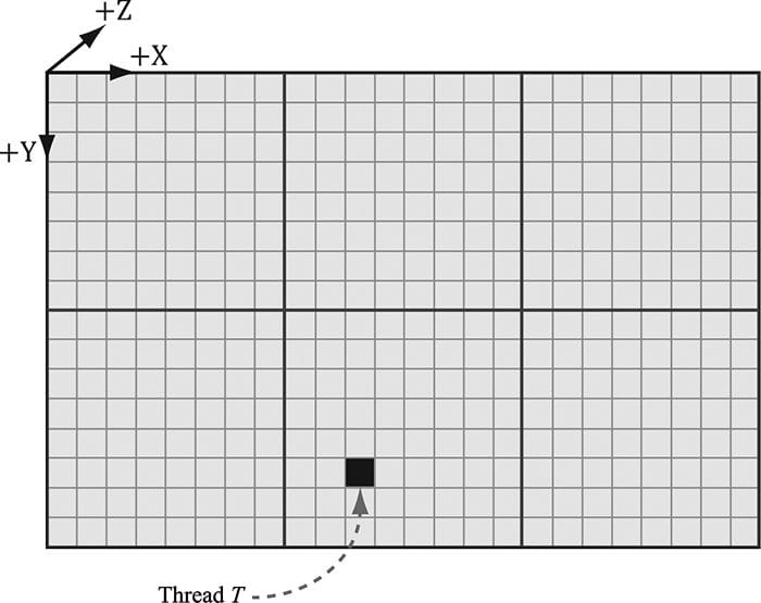
13.4 THREAD IDENTIFICATION SYSTEM VALUES

Consider Figure 13.4.

Figure 13.4. Consider the marked thread T. Thread T has thread group ID .(1, 1, 0). It has group thread ID (1, 5, 0). It has dispatch thread ID (1, 1, 0) ⊗ (8, 8, 0) + (2, 5, 0) = (10, 13, 0). It has group index ID 5·8 + 2 = 42.

1. Each thread group is assigned an ID by the system; this is called the group ID and has the system value semantic SV_GroupID. If G_x × G_y × G_z are the number of thread groups dispatched, then the group ID ranges from (0, 0, 0) to (G_x – 1, G_y – 1, G_z – 1).

2. Inside a thread group, each thread is given a unique ID relative to its group. If the thread group has size X × Y × Z, then the group thread IDs will range from (0, 0, 0) to (X – 1, Y – 1, Z – 1). The system value semantic for the group thread ID is SV_GroupThreadID.

3. A Dispatch call dispatches a grid of thread groups. The dispatch thread ID uniquely identifies a thread relative to all the threads generated by a Dispatch call. In other words, whereas the group thread ID uniquely identifies a thread relative to its thread group, the dispatch thread ID uniquely identifies a thread relative to the union of all the threads from all the thread groups dispatched by a Dispatch call. Let, ThreadGroupSize = (X,Y,Z) be the thread group size, then the dispatch thread ID can be derived from the group ID and the group thread ID as follows:

dispatchThreadID.xyz = groupID.xyz * ThreadGroupSize.xyz + groupThreadID.xyz;

The dispatch thread ID has the system value semantic SV_DispatchThreadID. If 3 × 2 thread groups are dispatched, where each thread group is 10 ×10, then a total of 60 threads are dispatched and the dispatch thread IDs will range from (0, 0, 0) to (29, 19, 0).

4. A linear index version of the group thread ID is given to us by Direct3D through the SV_GroupIndex system value; it is computed as:

groupIndex = groupThreadID.z*ThreadGroupSize.x*ThreadGroupSize.y +

groupThreadID.y*ThreadGroupSize.x + groupThreadID.x;

So why do we need these thread ID values. Well a compute shader generally takes some input data structure and outputs to some data structure. We can use the thread ID values as indexes into these data structures:

Texture2D gInputA;

Texture2D gInputB;

RWTexture2D<float4> gOutput;

[numthreads(16, 16, 1)]

void CS(int3 dispatchThreadID : SV_DispatchThreadID)

{

// Use dispatch thread ID to index into output and input textures.

gOutput[dispatchThreadID.xy] =

gInputA[dispatchThreadID.xy] +

gInputB[dispatchThreadID.xy];

}

The SV_GroupThreadID is useful for indexing into thread local storage memory (§13.6).

13.5 APPEND AND CONSUME BUFFERS

Suppose we have a buffer of particles defined by the structure:

struct Particle

{

float3 Position;

float3 Velocity;

float3 Acceleration;

};

and we want to update the particle positions based on their constant acceleration and velocity in the compute shader. Moreover, suppose that we do not care about the order the particles are updated nor the order they are written to the output buffer. Consume and append structured buffers are ideal for this scenario, and they provide the convenience that we do not have to worry about indexing:

struct Particle

{

float3 Position;

float3 Velocity;

float3 Acceleration;

};

float TimeStep = 1.0f / 60.0f;

ConsumeStructuredBuffer<Particle> gInput;

AppendStructuredBuffer<Particle> gOutput;

[numthreads(16, 16, 1)]

void CS()

{

// Consume a data element from the input buffer.

Particle p = gInput.Consume();

p.Velocity += p.Acceleration*TimeStep;

p.Position += p.Velocity*TimeStep;

// Append normalized vector to output buffer.

gOutput.Append( p );

}

Once a data element is consumed, it cannot be consumed again by a different thread; one thread will consume exactly one data element. And again, we emphasize that the order elements are consumed and appended are unknown; therefore, it is generally not the case that the ith element in the input buffer gets written to the ith element in the output buffer.

13.6 SHARED MEMORY AND SYNCHRONIZATION

Thread groups are given a section of so-called shared memory or thread local storage. Accessing this memory is fast and can be thought of being as fast as a hardware cache. In the compute shader code, shared memory is declared like so:

groupshared float4 gCache[256];

The array size can be whatever you want, but the maximum size of group shared memory is 32kb. Because the shared memory is local to the thread group, it is indexed with the SV_ThreadGroupID; so, for example, you might give each thread in the group access to one slot in the shared memory.

Using too much shared memory can lead to performance issues [Fung10], as the following example illustrates. Suppose a multiprocessor supports 32kb of shared memory, and your compute shader requires 20kb of shared memory. This means that only one thread group will fit on the multiprocessor because there is not enough memory left for another thread group [Fung10], as 20kb + 20kb = 40kb > 32kb. This limits the parallelism of the GPU, as a multiprocessor cannot switch off between thread groups to hide latency (recall from §13.1 that at least two thread groups per multiprocessor is recommended). Thus, even though the hardware technically supports 32kb of shared memory, performance improvements can be achieved by using less.

A common application of shared memory is to store texture values in it. Certain algorithms, such as blurs, require fetching the same texel multiple times. Sampling textures is actually one of the slower GPU operations because memory bandwidth and memory latency have not improved as much as the raw computational power of GPUs [Möller08]. A thread group can avoid redundant texture fetches by preloading all the needed texture samples into the shared memory array. The algorithm then proceeds to look up the texture samples in the shared memory array, which is very fast. Suppose we implement this strategy with the following erroneous code:

Texture2D gInput;

RWTexture2D<float4> gOutput;

groupshared float4 gCache[256];

[numthreads(256, 1, 1)]

void CS(int3 groupThreadID : SV_GroupThreadID,

int3 dispatchThreadID : SV_DispatchThreadID)

{

// Each thread samples the texture and stores the

// value in shared memory.

gCache[groupThreadID.x] = gInput[dispatchThreadID.xy];

// Do computation work: Access elements in shared memory

// that other threads stored:

// BAD!!! Left and right neighbor threads might not have

// finished sampling tzZhe texture and storing it in shared memory.

float4 left = gCache[groupThreadID.x - 1];

float4 right = gCache[groupThreadID.x + 1];

…

}

A problem arises with this scenario because we have no guarantee that all the threads in the thread group finish at the same time. Thus a thread could go to access a shared memory element that is not yet initialized because the neighboring threads responsible for initializing those elements have not finished yet. To fix this problem, before the compute shader can continue, it must wait until all the threads have done their texture loading into shared memory. This is accomplished by a synchronization command:

Texture2D gInput;

RWTexture2D<float4> gOutput;

groupshared float4 gCache[256];

[numthreads(256, 1, 1)]

void CS(int3 groupThreadID : SV_GroupThreadID,

int3 dispatchThreadID : SV_DispatchThreadID)

{

// Each thread samples the texture and stores the

// value in shared memory.

gCache[groupThreadID.x] = gInput[dispatchThreadID.xy];

// Wait for all threads in group to finish.

GroupMemoryBarrierWithGroupSync();

// Safe now to read any element in the shared memory

//and do computation work.

float4 left = gCache[groupThreadID.x - 1];

float4 right = gCache[groupThreadID.x + 1];

…

}

13.7 BLUR DEMO

In this section, we explain how to implement a blur algorithm on the compute shader. We begin by describing the mathematical theory of blurring. Then we discuss the technique of technique of render-to-texture, which our demo uses to generate a source image to blur. Finally, we review the code for a compute shader implementation and discuss how to handle certain details that make the implementation a little tricky.

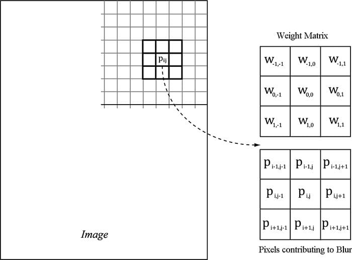
Figure 13.5. To blur the pixel Pij we compute the weighted average of the m × n matrix of pixels centered about the pixel. In this example, the matrix is a square 3 × 3 matrix, with blur radius a = b = 1. Observe that the center weight w₀₀ aligns with the pixel P_ij.

13.7.1 Blurring Theory

The blurring algorithm we use is described as follows: For each pixel P_ij. in the source image, compute the weighted average of the m × n matrix of pixels centered about the pixel P_ij (see Figure 13.5); this weighted average becomes the ijth pixel in the blurred image. Mathematically,

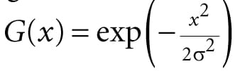
where m = 2a + 1 and n = 2b + 1. By forcing m and n to be odd, we ensure that the m × n matrix always has a natural “center.” We call a the vertical blur radius and b the horizontal blur radius. If a = b, then we just refer to the blur radius without having to specify the dimension. The m × n matrix of weights is called the blur kernel. Observe also that the weights must sum to 1. If the sum of the weights is less than one, the blurred image will appear darker as color has been removed. If the sum of the weights is greater than one, the blurred image will appear brighter as color has been added.

There are various ways to compute the weights so long as they sum to 1. A well-known blur operator found in many image editing programs is the Gaussian blur, which obtains its weights from the Gaussian function

. A graph of this function is shown in Figure 13.6 for different σ.

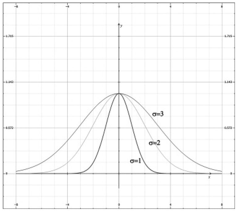
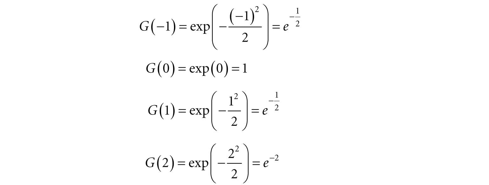
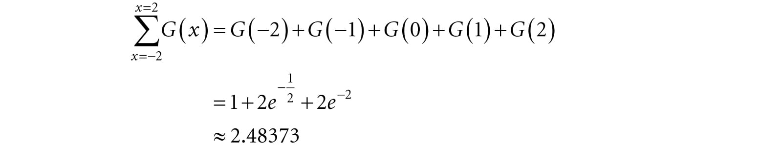
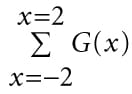
Figure 13.6. Plot of G(x) for σ = 1, 2, 3. Observe that a larger σ flattens the curve out and gives more weight to the neighboring points.

Let us suppose we are doing a 1 × 5 Gaussian blur (i.e., a 1D blur in the horizontal direction), and let σ = 1. Evaluating G(x) for x = −2, −1, 0, 1, 2 we have:

However, these values are not the weights because they do not sum to 1:

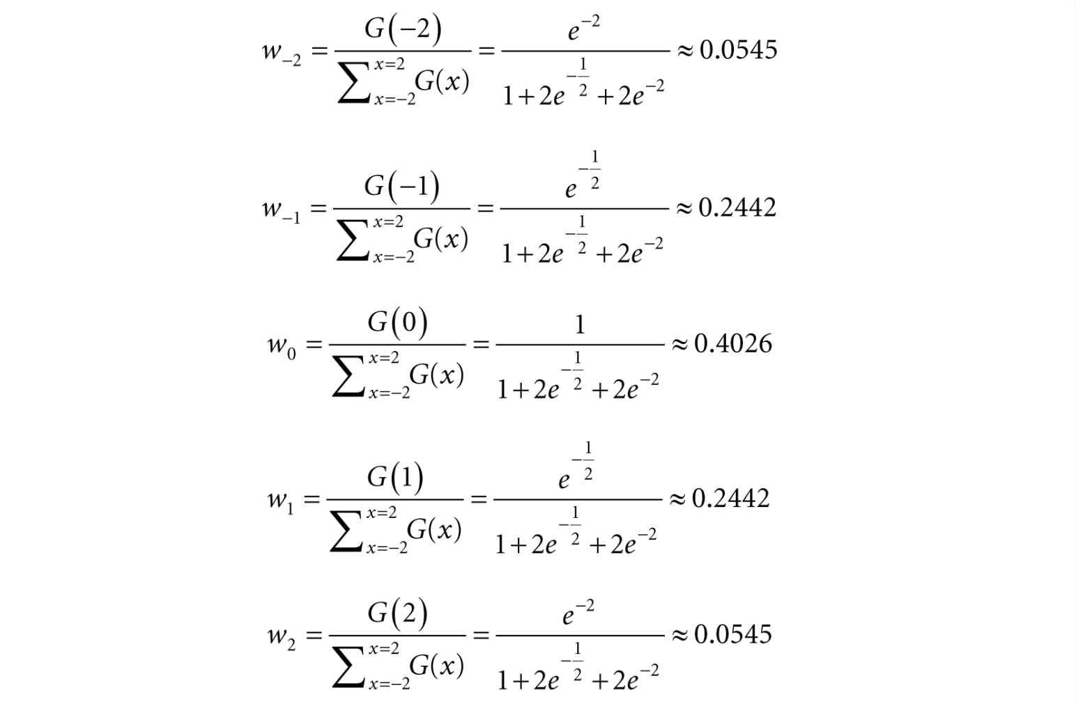
If we normalize the above equation by dividing by the sum

, then we obtain weights based on the Gaussian function that sum to 1:

Therefore, the Gaussian blur weights are:

The Gaussian blur is known to be separable, which means it can be broken up into two 1D blurs as follows.

1. Blur the input image I using a 1D horizontal blur: I_H = Blur_H ( I ).

2. Blur the output from the previous step using a 1D vertical blur: Blur ( I ) = Blur_V ( I_H ).

Written more succinctly, we have:

Suppose that the blur kernel is a 9 × 9 matrix, so that we needed a total of 81 samples to do the 2D blur. By separating the blur into two 1D blurs, we only need 9 + 9 = 18 samples. Typically, we will be blurring textures; as mentioned in this chapter, fetching texture samples is expensive, so reducing texture samples by separating a blur is a welcome improvement. Even if a blur is not separable (some blur operators are not), we can often make the simplification and assume it is for the sake of performance, as long as the final image looks accurate enough.

13.7.2 Render-to-Texture

So far in our programs, we have been rendering to the back buffer. But what is the back buffer? If we review our D3DApp code, we see that the back buffer is just a texture in the swap chain:

Microsoft::WRL::ComPtr<ID3D12Resource> mSwapChainBuffer[SwapChainBufferCount];

CD3DX12_CPU_DESCRIPTOR_HANDLE rtvHeapHandle(mRtvHeap->GetCPUDescriptorHandleForHeapStart());

for (UINT i = 0; i < SwapChainBufferCount; i++)

{

ThrowIfFailed(mSwapChain->GetBuffer(i,

IID_PPV_ARGS(&mSwapChainBuffer[i])));

md3dDevice->CreateRenderTargetView(

mSwapChainBuffer[i].Get(), nullptr, rtvHeapHandle);

rtvHeapHandle.Offset(1, mRtvDescriptorSize);

}

We instruct Direct3D to render to the back buffer by binding a render target view of the back buffer to the OM stage of the rendering pipeline:

// Specify the buffers we are going to render to.

mCommandList->OMSetRenderTargets(1, &CurrentBackBufferView(),

true, &DepthStencilView());

The contents of the back buffer are eventually displayed on the screen when the back buffer is presented via the IDXGISwapChain::Present method.

If we think about this code, there is nothing that stops us from creating another texture, creating a render target view to it, and binding it to the OM stage of the rendering pipeline. Thus we will be drawing to this different “off-screen” texture (possible with a different camera) instead of the back buffer. This technique is known as render-to-off-screen-texture or simply render-to-texture. The only difference is that since this texture is not the back buffer, it does not get displayed to the screen during presentation.

Figure 13.7. A camera is placed above the player from a bird’s eye view and renders the scene into an off-screen texture. When we draw the scene from the player’s eye to the back buffer, we map the texture onto a quad in the bottom-right corner of the screen to display the radar map.

Consequently, render-to-texture might seem worthless at first as it does not get presented to the screen. But, after we have rendered-to-texture, we can bind the back buffer back to the OM stage, and resume drawing geometry to the back buffer. We can texture the geometry with the texture we generated during the render-to-texture period. This strategy is used to implement a variety of special effects. For example, you can render-to-texture the scene from a bird’s eye view to a texture. Then, when drawing to the back buffer, you can draw a quad in the lower-right corner of the screen with the bird’s eye view texture to simulate a radar system (see Figure 13.7). Other render-to-texture techniques include:

1. Shadow mapping

2. Screen Space Ambient Occlusion

3. Dynamic reflections with cube maps

Using render-to-texture, implementing a blurring algorithm on the GPU would work the following way: render our normal demo scene to an off-screen texture. This texture will be the input into our blurring algorithm that executes on the compute shader. After the texture is blurred, we will draw a full screen quad to the back buffer with the blurred texture applied so that we can see the blurred result to test our blur implementation. The steps are outlined as follows:

1. Draw scene as usual to an off-screen texture.

2. Blur the off-screen texture using a compute shader program.

3. Restore the back buffer as the render target, and draw a full screen quad with the blurred texture applied.

Using render-to-texture to implement a blur works fine, and is the required approach if we want to render the scene to a different sized texture than the back buffer. However, if we make the assumption that our off-screen textures match the format and size of our back buffer, instead of redirecting rendering to our off-screen texture, we can render to the back buffer as usual, and then do a CopyResource to copy the back-buffer contents to our off-screen texture. Then we can do our compute work on our off-screen textures, and then draw a full-screen quad to the back buffer with the blurred texture to produce the final screen output.

// Copy the input (back-buffer in this example) to BlurMap0.

cmdList->CopyResource(mBlurMap0.Get(), input);

This is the technique we will use to implement our blur demo, but Exercise 6 asks you to implement a different filter using render-to-texture.

13.7.3 Blur Implementation Overview

We assume that the blur is separable, so we break the blur down into computing two 1D blurs—a horizontal one and a vertical one. Implementing this requires two texture buffers where we can read and write to both; therefore, we need a SRV and UAV to both textures. Let us call one of the textures A and the other texture B. The blurring algorithm proceeds as follows:

1. Bind the SRV to A as an input to the compute shader (this is the input image that will be horizontally blurred).

2. Bind the UAV to B as an output to the compute shader (this is the output image that will store the blurred result).

3. Dispatch the thread groups to perform the horizontal blur operation. After this, texture B stores the horizontally blurred result Blur_H(I), where I is the image to blur.

4. Bind the SRV to B as an input to the compute shader (this is the horizontally blurred image that will next be vertically blurred).

5. Bind the UAV to A as an output to the compute shader (this is the output image that will store the final blurred result).

6. Dispatch the thread groups to perform the vertical blur operation. After this, texture A stores the final blurred result Blur (I), where I is the image to blur.

This logic implements the separable blur formula Blur(I) = Blur_V(Blur_H(I)). Observe that both texture A and texture B serve as an input and an output to the compute shader at some point, but not simultaneously. (It is Direct3D error to bind a resource as an input and output at the same time.) The combined horizontal and vertical blur passes constitute one complete blur pass. The resulting image can be blurred further by performing another blur pass on it. We can repeatedly blur an image until the image is blurred to the desired level.

The texture we render the scene to has the same resolution as the window client area. Therefore, we need to rebuild the off-screen texture, as well as the second texture buffer B used in the blur algorithm. We do this on the OnResize method:

void BlurApp::OnResize()

{

D3DApp::OnResize();

// The window resized, so update the aspect ratio and

// recompute the projection matrix.

XMMATRIX P = XMMatrixPerspectiveFovLH(

0.25f*MathHelper::Pi, AspectRatio(),

1.0f, 1000.0f);

XMStoreFloat4x4(&mProj, P);

if(mBlurFilter != nullptr)

{

mBlurFilter->OnResize(mClientWidth, mClientHeight);

}

}

void BlurFilter::OnResize(UINT newWidth, UINT newHeight)

{

if((mWidth != newWidth) || (mHeight != newHeight))

{

mWidth = newWidth;

mHeight = newHeight;

// Rebuild the off-screen texture resource with new dimensions.

BuildResources();

// New resources, so we need new descriptors to that resource.

BuildDescriptors();

}

}

The mBlur variable is an instance of a BlurFilter helper class we make. This class encapsulates the texture resources to textures A and B, encapsulates SRVs and UAVs to the textures, and provides a method that kicks off the actual blur operation on the compute shader, the implementation of which we will see in a moment.

The BlurFilter class encapsulates texture resources. To bind these resources to the pipeline to use for a draw/dispatch command, we are going to need to create descriptors to these resources. That means we will have to allocate extra room in the D3D12_DESCRIPTOR_HEAP_TYPE_CBV_SRV_UAV descriptor heap to store these descriptors. The BlurFilter::BuildDescriptors method takes descriptor handles to the starting location in the descriptor heap to store the descriptors used by BlurFilter. The method caches the handles for all the descriptors it needs and then creates the corresponding descriptors. The reason it caches the handles is so that it can recreate the descriptors when the resources change, which happens when the screen is resized:

void BlurFilter::BuildDescriptors(

CD3DX12_CPU_DESCRIPTOR_HANDLE hCpuDescriptor,

CD3DX12_GPU_DESCRIPTOR_HANDLE hGpuDescriptor,

UINT descriptorSize)

{

// Save references to the descriptors.

mBlur0CpuSrv = hCpuDescriptor;

mBlur0CpuUav = hCpuDescriptor.Offset(1, descriptorSize);

mBlur1CpuSrv = hCpuDescriptor.Offset(1, descriptorSize);

mBlur1CpuUav = hCpuDescriptor.Offset(1, descriptorSize);

mBlur0GpuSrv = hGpuDescriptor;

mBlur0GpuUav = hGpuDescriptor.Offset(1, descriptorSize);

mBlur1GpuSrv = hGpuDescriptor.Offset(1, descriptorSize);

mBlur1GpuUav = hGpuDescriptor.Offset(1, descriptorSize);

BuildDescriptors();

}

void BlurFilter::BuildDescriptors()

{

D3D12_SHADER_RESOURCE_VIEW_DESC srvDesc = {};

srvDesc.Shader4ComponentMapping = D3D12_DEFAULT_SHADER_4_COMPONENT_MAPPING;

srvDesc.Format = mFormat;

srvDesc.ViewDimension = D3D12_SRV_DIMENSION_TEXTURE2D;

srvDesc.Texture2D.MostDetailedMip = 0;

srvDesc.Texture2D.MipLevels = 1;

D3D12_UNORDERED_ACCESS_VIEW_DESC uavDesc = {};

uavDesc.Format = mFormat;

uavDesc.ViewDimension = D3D12_UAV_DIMENSION_TEXTURE2D;

uavDesc.Texture2D.MipSlice = 0;

md3dDevice->CreateShaderResourceView(mBlurMap0.Get(), &srvDesc, mBlur0CpuSrv);

md3dDevice->CreateUnorderedAccessView(mBlurMap0.Get(),

nullptr, &uavDesc, mBlur0CpuUav);

md3dDevice->CreateShaderResourceView(mBlurMap1.Get(), &srvDesc, mBlur1CpuSrv);

md3dDevice->CreateUnorderedAccessView(mBlurMap1.Get(),

nullptr, &uavDesc, mBlur1CpuUav);

}

// In BlurApp.cpp…Offset to location in heap to

// store descriptors for BlurFilter

mBlurFilter->BuildDescriptors(

CD3DX12_CPU_DESCRIPTOR_HANDLE(

mCbvSrvUavDescriptorHeap->GetCPUDescriptorHandleForHeapStart(),

3, mCbvSrvUavDescriptorSize),

CD3DX12_GPU_DESCRIPTOR_HANDLE(

mCbvSrvUavDescriptorHeap->GetGPUDescriptorHandleForHeapStart(),

3, mCbvSrvUavDescriptorSize),

mCbvSrvUavDescriptorSize);

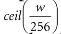
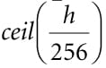
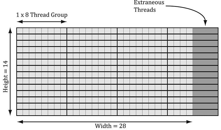
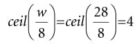
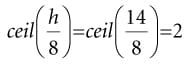
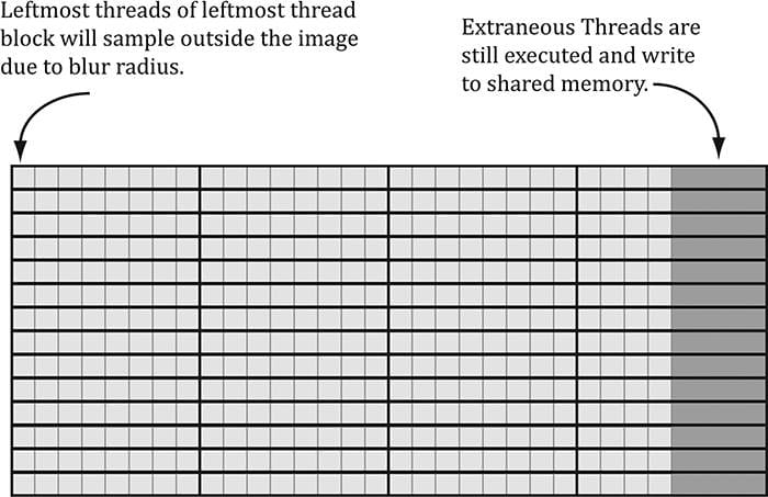
Suppose our image has width w and height h. As we will see in the next section when we look at the compute shader, for the horizontal 1D blur, our thread group is a horizontal line segment of 256 threads, and each thread is responsible for blurring one pixel in the image. Therefore, we need to dispatch

thread groups in the x-direction and h thread groups in the y-direction in order for each pixel in the image to be blurred. If 256 does not divide evenly into w, the last horizontal thread group will have extraneous threads (see Figure (13.8)). There is not really anything we can do about this since the thread group size is fixed. We take care of out-of-bounds with clamping checks in the shader code.

The situation is similar for the vertical 1D blur. Again, our thread group is a vertical line segment of 256 threads, and each thread is responsible for blurring one pixel in the image. Therefore, we need to dispatch

thread groups in the y-direction and w thread groups in the x-direction in order for each pixel in the image to be blurred.

The code below figures out how many thread groups to dispatch in each direction, and kicks off the actual blur operation on the compute shader:

void BlurFilter::Execute(ID3D12GraphicsCommandList* cmdList,

ID3D12RootSignature* rootSig,

ID3D12PipelineState* horzBlurPSO,

ID3D12PipelineState* vertBlurPSO,

ID3D12Resource* input,

int blurCount)

{

auto weights = CalcGaussWeights(2.5f);

int blurRadius = (int)weights.size() / 2;

cmdList->SetComputeRootSignature(rootSig);

cmdList->SetComputeRoot32BitConstants(0, 1, &blurRadius, 0);

cmdList->SetComputeRoot32BitConstants(0, (UINT)weights.size(), weights.

data(), 1);

cmdList->ResourceBarrier(1, &CD3DX12_RESOURCE_BARRIER::Transition(input,

D3D12_RESOURCE_STATE_RENDER_TARGET, D3D12_RESOURCE_STATE_COPY_SOURCE));

cmdList->ResourceBarrier(1, &CD3DX12_RESOURCE_BARRIER::Transition(mBlurMap0.

Get(),

D3D12_RESOURCE_STATE_COMMON, D3D12_RESOURCE_STATE_COPY_DEST));

// Copy the input (back-buffer in this example) to BlurMap0.

cmdList->CopyResource(mBlurMap0.Get(), input);

cmdList->ResourceBarrier(1, &CD3DX12_RESOURCE_BARRIER::Transition(mBlurMap0.

Get(),

D3D12_RESOURCE_STATE_COPY_DEST, D3D12_RESOURCE_STATE_GENERIC_READ));

cmdList->ResourceBarrier(1, &CD3DX12_RESOURCE_BARRIER::Transition(mBlurMap1.

Get(),

D3D12_RESOURCE_STATE_COMMON, D3D12_RESOURCE_STATE_UNORDERED_ACCESS));

for(int i = 0; i < blurCount; ++i)

{

//

// Horizontal Blur pass.

//

cmdList->SetPipelineState(horzBlurPSO);

cmdList->SetComputeRootDescriptorTable(1, mBlur0GpuSrv);

cmdList->SetComputeRootDescriptorTable(2, mBlur1GpuUav);

// How many groups do we need to dispatch to cover a row of pixels, where

// each group covers 256 pixels (the 256 is defined in the ComputeShader).

UINT numGroupsX = (UINT)ceilf(mWidth / 256.0f);

cmdList->Dispatch(numGroupsX, mHeight, 1);

cmdList->ResourceBarrier(1, &CD3DX12_RESOURCE_BARRIER::Transition(

mBlurMap0.Get(),

D3D12_RESOURCE_STATE_GENERIC_READ,

D3D12_RESOURCE_STATE_UNORDERED_ACCESS));

cmdList->ResourceBarrier(1, &CD3DX12_RESOURCE_BARRIER::Transition(

mBlurMap1.Get(),

D3D12_RESOURCE_STATE_UNORDERED_ACCESS,

D3D12_RESOURCE_STATE_GENERIC_READ));

//

// Vertical Blur pass.

//

cmdList->SetPipelineState(vertBlurPSO);

cmdList->SetComputeRootDescriptorTable(1, mBlur1GpuSrv);

cmdList->SetComputeRootDescriptorTable(2, mBlur0GpuUav);

// How many groups do we need to dispatch to cover a column of pixels,

// where each group covers 256 pixels (the 256 is defined in the

// ComputeShader).

UINT numGroupsY = (UINT)ceilf(mHeight / 256.0f);

cmdList->Dispatch(mWidth, numGroupsY, 1);

cmdList->ResourceBarrier(1, &CD3DX12_RESOURCE_BARRIER::Transition(

mBlurMap0.Get(),

D3D12_RESOURCE_STATE_UNORDERED_ACCESS,

D3D12_RESOURCE_STATE_GENERIC_READ));

cmdList->ResourceBarrier(1, &CD3DX12_RESOURCE_BARRIER::Transition(

mBlurMap1.Get(),

D3D12_RESOURCE_STATE_GENERIC_READ,

D3D12_RESOURCE_STATE_UNORDERED_ACCESS));

}

}

Figure 13.8. Consider a 28 × 14 texture, where our horizontal thread groups are 8 × 1 and our vertical thread groups are 1 × 8 (X × Y format). For the horizontal pass, in order to cover all the pixels we need to dispatch

thread groups in the x-direction and 14 thread groups in the y-direction. Since 28 is not a multiple of 8, we end of with extraneous threads that do not do any work in the right-most thread groups. For the vertical pass, in order to cover all the pixels we need to dispatch

thread groups in the y-direction and 28 thread groups in the x-direction. Since 14 is not a multiple of 8, we end up with extraneous threads that do not do any work in the bottom-most thread groups. The same concepts apply to a larger texture with thread groups of size 256.

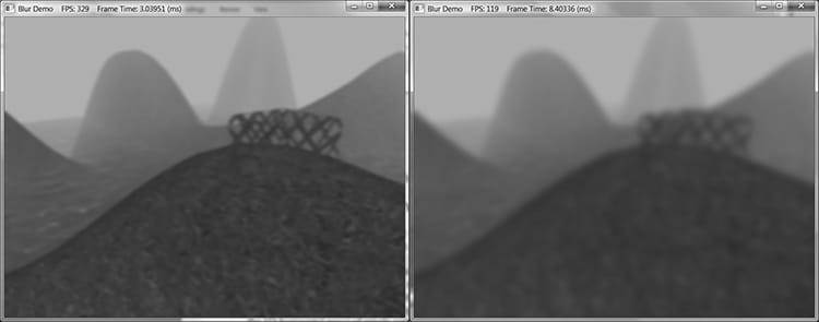
Figure 13.9. Left: A screenshot of the “Blur” demo where the image has been blurred two times. Right: A screen shot of the “Blur” demo where the image has been blurred eight times.

13.7.4 Compute Shader Program

In this section, we look the compute shader program that actually does the blurring. We will only discuss the horizontal blur case. The vertical blur case is analogous, but the situation transposed.

As mentioned in the previous section, our thread group is a horizontal line segment of 256 threads, and each thread is responsible for blurring one pixel in the image. An inefficient first approach is to just implement the blur algorithm directly. That is, each thread simply performs the weighted average of the row matrix (row matrix because we are doing the 1D horizontal pass) of pixels centered about the pixel the thread is processing. The problem with this approach is that it requires fetching the same texel multiple times (see Figure 13.10).

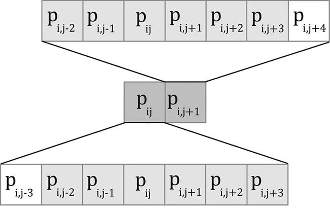
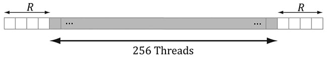
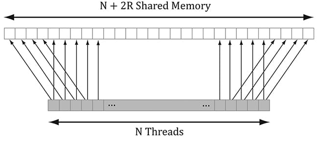
Figure 13.10. Consider just two neighboring pixels in the input image, and suppose that the blur kernel is 1 × 7. Observe that six out of the eight unique pixels are sampled twice—once for each pixel.

We can optimize by following the strategy described in §13.6 and take advantage of shared memory. Each thread can read in a texel value and store it in shared memory. After all the threads are done reading their texel values into shared memory, the threads can proceed to perform the blur, but where it reads the texels from the shared memory, which is fast to access. The only tricky thing about this is that a thread group of n = 256 threads requires n + 2R texels to perform the blur, where R is the blur radius (Figure 13.11).

Figure 13.11. Pixels near the boundaries of the thread group will read pixels outside the thread group due to the blur radius.

The solution is simple; we allocate n + 2R elements of shared memory, and have 2R threads lookup two texel values. The only thing that is tricky about this is that it requires a little more book keeping when indexing into the shared memory; we no longer have the ith group thread ID corresponding to the ith element in the shared memory. Figure 13.12 shows the mapping from threads to shared memory for R = 4.

Figure 13.12. In this example, R = 4. The four leftmost threads each read two texel values and store them into shared memory. The four rightmost threads each read two texel values and store them into shared memory. Every other thread just reads one texel value and stores it in shared memory. This gives us all the texel values we need to blur N pixels with blur radius R.

Finally, the last situation to discuss is that the left-most thread group and the right-most thread group can index the input image out-of-bounds, as shown in Figure 13.13.

Figure 13.13. Situations where we can read outside the bounds of the image

Reading from an out-of-bounds index is not illegal—it is defined to return 0 (and writing to an out-of-bounds index results in a no-op). However, we do not want to read 0 when we go out-of-bounds, as it means 0 colors (i.e., black) will make their way into the blur at the boundaries. Instead, we want to implement something analogous to the clamp texture address mode, where if we read an out-of-bounds value, it returns the same value as the boundary texel. This can be implemented by clamping the indices:

// Clamp out of bound samples that occur at left image borders.

int x = max(dispatchThreadID.x - gBlurRadius, 0);

gCache[groupThreadID.x] = gInput[int2(x, dispatchThreadID.y)];

// Clamp out of bound samples that occur at right image borders.

int x = min(dispatchThreadID.x + gBlurRadius, gInput.Length.x-1);

gCache[groupThreadID.x+2*gBlurRadius] =

gInput[int2(x, dispatchThreadID.y)];

// Clamp out of bound samples that occur at image borders.

gCache[groupThreadID.x+gBlurRadius] =

gInput[min(dispatchThreadID.xy, gInput.Length.xy-1)];

The full shader code is shown below:

//====================================================================

// Performs a separable Guassian blur with a blur radius up to 5 pixels.

//====================================================================

cbuffer cbSettings : register(b0)

{

// We cannot have an array entry in a constant buffer that gets mapped onto

// root constants, so list each element.

int gBlurRadius;

// Support up to 11 blur weights.

float w0;

float w1;

float w2;

float w3;

float w4;

float w5;

float w6;

float w7;

float w8;

float w9;

float w10;

};

static const int gMaxBlurRadius = 5;

Texture2D gInput : register(t0);

RWTexture2D<float4> gOutput : register(u0);

#define N 256

#define CacheSize (N + 2*gMaxBlurRadius)

groupshared float4 gCache[CacheSize];

[numthreads(N, 1, 1)]

void HorzBlurCS(int3 groupThreadID : SV_GroupThreadID,

int3 dispatchThreadID : SV_DispatchThreadID)

{

// Put in an array for each indexing.

float weights[11] = { w0, w1, w2, w3, w4, w5, w6, w7, w8, w9, w10 };

//

// Fill local thread storage to reduce bandwidth. To blur

// N pixels, we will need to load N + 2*BlurRadius pixels

// due to the blur radius.

//

// This thread group runs N threads. To get the extra 2*BlurRadius

// pixels, have 2*BlurRadius threads sample an extra pixel.

if(groupThreadID.x < gBlurRadius)

{

// Clamp out of bound samples that occur at image borders.

int x = max(dispatchThreadID.x - gBlurRadius, 0);

gCache[groupThreadID.x] = gInput[int2(x, dispatchThreadID.y)];

}

if(groupThreadID.x >= N-gBlurRadius)

{

// Clamp out of bound samples that occur at image borders.

int x = min(dispatchThreadID.x + gBlurRadius, gInput.Length.x-1);

gCache[groupThreadID.x+2*gBlurRadius] = gInput[int2(x, dispatchThreadID.y)];

}

// Clamp out of bound samples that occur at image borders.

gCache[groupThreadID.x+gBlurRadius] = gInput[min(dispatchThreadID.xy, gInput.Length.xy-1)];

// Wait for all threads to finish.

GroupMemoryBarrierWithGroupSync();

//

// Now blur each pixel.

//

float4 blurColor = float4(0, 0, 0, 0);

for(int i = -gBlurRadius; i <= gBlurRadius; ++i)

{

int k = groupThreadID.x + gBlurRadius + i;

blurColor += weights[i+gBlurRadius]*gCache[k];

}

gOutput[dispatchThreadID.xy] = blurColor;

}

[numthreads(1, N, 1)]

void VertBlurCS(int3 groupThreadID : SV_GroupThreadID,

int3 dispatchThreadID : SV_DispatchThreadID)

{

// Put in an array for each indexing.

float weights[11] = { w0, w1, w2, w3, w4, w5, w6, w7, w8, w9, w10 };

//

// Fill local thread storage to reduce bandwidth. To blur

// N pixels, we will need to load N + 2*BlurRadius pixels

// due to the blur radius.

//

// This thread group runs N threads. To get the extra 2*BlurRadius

// pixels, have 2*BlurRadius threads sample an extra pixel.

if(groupThreadID.y < gBlurRadius)

{

// Clamp out of bound samples that occur at image borders.

int y = max(dispatchThreadID.y - gBlurRadius, 0);

gCache[groupThreadID.y] = gInput[int2(dispatchThreadID.x, y)];

}

if(groupThreadID.y >= N-gBlurRadius)

{

// Clamp out of bound samples that occur at image borders.

int y = min(dispatchThreadID.y + gBlurRadius, gInput.Length.y-1);

gCache[groupThreadID.y+2*gBlurRadius] = gInput[int2(dispatchThreadID.x, y)];

}

// Clamp out of bound samples that occur at image borders.

gCache[groupThreadID.y+gBlurRadius] = gInput[min(dispatchThreadID.xy,

gInput.Length.xy-1)];

// Wait for all threads to finish.

GroupMemoryBarrierWithGroupSync();

//

// Now blur each pixel.

//

float4 blurColor = float4(0, 0, 0, 0);

for(int i = -gBlurRadius; i <= gBlurRadius; ++i)

{

int k = groupThreadID.y + gBlurRadius + i;

blurColor += weights[i+gBlurRadius]*gCache[k];

}

gOutput[dispatchThreadID.xy] = blurColor;

}

For the last line

gOutput[dispatchThreadID.xy] = blurColor;

it is possible in the right-most thread group to have extraneous threads that do not correspond to an element in the output texture (Figure 13.13). That is, the dispatchThreadID.xy will be an out-of-bounds index for the output texture. However, we do not need to worry about handling this case, as an out-of-bound write results in a no-op.

13.8 FURTHER RESOURCES

Compute shader programming is a subject in its own right, and there are several books on using GPUs for compute programs:

1. Programming Massively Parallel Processors: A Hands-on Approach by David B. Kirk and Wen-mei W. Hwu.

2. OpenCL Programming Guide by Aaftab Munshi, Benedict R. Gaster, Timothy G. Mattson, James Fung, and Dan Ginsburg.

Technologies like CUDA and OpenCL are just different APIs for accessing the GPU for writing compute programs. Best practices for CUDA and OpenCL programs are also best practices for Direct Compute programs, as the programs are all executed on the same hardware. In this chapter, we have shown the majority of Direct Compute syntax, and so you should have no trouble porting a CUDA or OpenCL program to Direct Compute.

Chuck Walbourn has posted a blog page consisting of links to many Direct Compute presentations:

http://blogs.msdn.com/b/chuckw/archive/2010/07/14/directcompute.aspx

In addition, Microsoft’s Channel 9 has a series of lecture videos on Direct Compute programming:

http://channel9.msdn.com/tags/DirectCompute-Lecture-Series/

Finally, NVIDIA has a whole section on CUDA training.

http://developer.nvidia.com/cuda-training

In particular, there are full video lectures on CUDA programming from the University of Illinois, which we highly recommend. Again, we emphasize that CUDA is just another API for accessing the compute functionality of the GPU. Once you understand the syntax, the hard part about GPU computing is learning how to write efficient programs for it. By studying these lectures on CUDA, you will get a better idea of how GPU hardware works so that you can write optimal code.

13.9 SUMMARY

1. The ID3D12GraphicsCommandList::Dispatch API call dispatches a grid of thread groups. Each thread group is a 3D grid of threads; the number of threads per thread group is specified by the [numthreads(x,y,z)] attribute in the compute shader. For performance reasons, the total number of threads should be a multiple of the warp size (thirty-two for NVIDIA hardware) or a multiple of the wavefront size (sixty-four ATI hardware).

2. To ensure parallelism, at least two thread groups should be dispatched per multiprocessor. So if your hardware has sixteen multiprocessors, then at least thirty-two thread groups should be dispatched so a multiprocessor always has work to do. Future hardware will likely have more multiprocessors, so the number of thread groups should be even higher to ensure your program scales well to future hardware.

3. Once thread groups are assigned to a multiprocessor, the threads in the thread groups are divided into warps of thirty-two threads on NVIDIA hardware. The multiprocessor than works on a warp of threads at a time in an SIMD fashion (i.e., the same instruction is executed for each thread in the warp). If a warp becomes stalled, say to fetch texture memory, the multiprocessor can quickly switch and execute instructions for another warp to hide this latency. This keeps the multiprocessor always busy. You can see why there is the recommendation of the thread group size being a multiple of the warp size; if it were not then when the thread group is divided into warps, there will be warps with threads that are not doing anything.

4. Texture resources can be accessed by the compute shader for input by creating a SRV to the texture and binding it to the compute shader. A read-write texture (RWTexture) is a texture the compute shader can read and write output to. To set a texture for reading and writing to the compute shader, a UAV (unordered access view) to the texture is created and bound to the compute shader. Texture elements can be indexed with operator [] notation, or sampled via texture coordinates and sampler state with the SampleLevel method.

5. A structured buffer is a buffer of elements that are all the same type, like an array. The type can be a user-defined type defined by a struct for example. Read-only structured buffers are defined in the HLSL like this:

StructuredBuffer<DataType> gInputA;

Read-write structured buffers are defined in the HLSL like this:

RWStructuredBuffer<DataType> gOutput;

Read-only buffer resources can be accessed by the compute shader for input by create a SRV to a structured buffer and binding it to the compute shader. Read-write buffer resources can be accessed by the compute shader for reading and writing by creating a UAV to a structured buffer and binding it to the compute shader.

6. Various thread IDs are passed into the compute shader via the system values. These IDs are often used to index into resources and shared memory.

7. Consume and append structured buffers are defined in the HLSL like this:

ConsumeStructuredBuffer<DataType> gInput;

AppendStructuredBuffer<DataType> gOutput;

Consume and append structured buffers are useful if you do not care about the order in which data elements are processed and written to the output buffer, as it allows you to avoid indexing syntax. Note that append buffers do not automatically grow, and they must have be large enough to store all the data elements you will append to it.

8. Thread groups are given a section of so-called shared memory or thread local storage. Accessing this memory is fast and can be thought of being as fast as a hardware cache. This shared memory cache can be useful for optimizations or needed for algorithm implementations. In the compute shader code, shared memory is declared like so:

groupshared float4 gCache[N];

The array size N can be whatever you want, but the maximum size of group shared memory is 32kb. Assuming a multiprocessor supports the maximum of 32kb for shared memory, for performance, a thread group should not use more than 16kb of shared memory; otherwise it is impossible to fit two thread groups on a single multiprocessor.

9. Avoid switching between compute processing and rendering when possible, as there is overhead required to make the switch. In general, for each frame try to do all of your compute work first, then do all of your rendering work.

13.10 EXERCISES

1. Write a compute shader that inputs a structured buffer of sixty-four 3D vectors with random magnitudes contained in [1, 10]. The compute shader computes the length of the vectors and outputs the result into a floating-point buffer. Copy the results to CPU memory and save the results to file. Verify that all the lengths are contained in [1, 10].

2. Redo the previous exercise using typed buffers; that is, Buffer<float3> for the input buffer and Buffer<float> for the output buffer.

3. Assume that in the previous exercises that we do not care the order in which the vectors are normalized. Redo Exercise 1 using Append and Consume buffers.

4. Research the bilateral blur technique and implement it on the compute shader. Redo the “Blur” demo using the bilateral blur.

5. So far in our demos we have done a 2D wave equation on the CPU with the Waves class in Waves.h/.cpp. Port this to a GPU implementation. Use textures of floats to store the previous, current, and next height solutions. Because UAVs are read/write, we can just use UAVs throughout and not bother with SRVs:

RWTexture2D<float> gPrevSolInput : register(u0);

RWTexture2D<float> gCurrSolInput : register(u1);

RWTexture2D<float> gOutput : register(u2);

Use the compute shader to perform the wave update computations. A separate compute shader can be used to disturb the water to generate waves. After you have update the grid heights, you can render a triangle grid with the same vertex resolution as the wave textures (so there is a texel corresponding to each grid vertex), and bind the current wave solution texture to a new “waves” vertex shader. Then in the vertex shader, you can sample the solution texture to offset the heights (this is called displacement mapping) and estimate the normal.

VertexOut VS(VertexIn vin)

{

VertexOut vout = (VertexOut)0.0f;

#ifdef DISPLACEMENT_MAP

// Sample the displacement map using non-transformed [0,1]^2 tex-coords.

vin.PosL.y += gDisplacementMap.SampleLevel(gsamLinearWrap, vin.TexC, 1.0f).r;

// Estimate normal using finite difference.

float du = gDisplacementMapTexelSize.x;

float dv = gDisplacementMapTexelSize.y;

float l = gDisplacementMap.SampleLevel( gsamPointClamp,

vin.TexC-float2(du, 0.0f), 0.0f ).r;

float r = gDisplacementMap.SampleLevel( gsamPointClamp,

vin.TexC+float2(du, 0.0f), 0.0f ).r;

float t = gDisplacementMap.SampleLevel( gsamPointClamp,

vin.TexC-float2(0.0f, dv), 0.0f ).r;

float b = gDisplacementMap.SampleLevel( gsamPointClamp,

vin.TexC+float2(0.0f, dv), 0.0f ).r;

vin.NormalL = normalize( float3(-r+l, 2.0f*gGridSpatialStep, b-t) );

#endif

// Transform to world space.

float4 posW = mul(float4(vin.PosL, 1.0f), gWorld);

vout.PosW = posW.xyz;

// Assumes nonuniform scaling; otherwise, need to use inverse-transpose of

// world matrix.

vout.NormalW = mul(vin.NormalL, (float3x3)gWorld);

// Transform to homogeneous clip space.

vout.PosH = mul(posW, gViewProj);

// Output vertex attributes for interpolation across triangle.

float4 texC = mul(float4(vin.TexC, 0.0f, 1.0f), gTexTransform);

vout.TexC = mul(texC, gMatTransform).xy;

return vout;

}

Compare your performance results (time per frame) to a CPU implementation with 512 × 512 grid points in release mode.

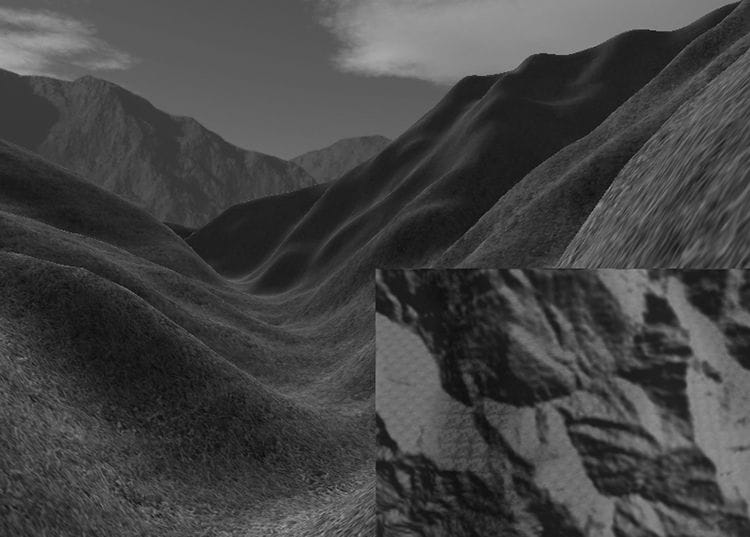
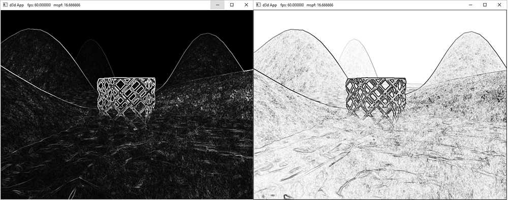
6. The Sobel Operator measures edges in an image. For each pixel, it estimates the magnitude of the gradient. A pixel with a large gradient magnitude means the color difference between the pixel and its neighbors has high variation, and so that pixel must be on an edge. A pixel with a small gradient magnitude means the color difference between the pixel and its neighbors has low variation, and so that pixel is not on an edge. Note that the Sobel Operator does not return a binary result (on edge or not on edge); it returns a grayscale value in the range [0, 1] that denotes an edge “steepness” amount, where 0 denotes no edge (the color is not changing locally about a pixel) and 1 denotes a very steep edge or discontinuity (the color is changing a lot locally about a pixel). The inverse Sobel image (1 − c) is often more useful, as white denotes no edge and black denotes edges (see Figure 13.14).

Figure 13.14. Left: In image after applying Sobel Operator, the white pixels denote edges. In the inverse image of the Sobel Operator, the black pixels denote edge.

If you color multiply the original image by the inverse of the image generated by the Sobel Operator, then you get a stylized cartoon/comic book like effect by making edges look like black pen strokes (see Figure 13.15). You can take this stylized cartoon/comic book effect even further by first blurring the original image to wash out details, then applying the Sobel Operator on the blurred image to build the edge detection image, and finally multiplying the blurred image by the inverse of the edge detection image.

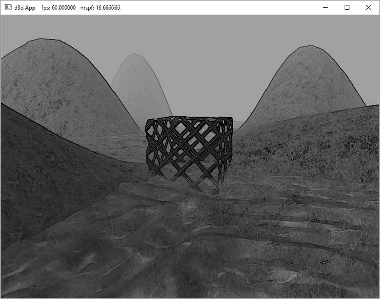
Figure 13.15. Multiplying the original image by the inverse of the edge detection image to produce a stylized look where edge look like black pen strokes

Use render-to-texture and a compute shader to implement the Sobel Operator. After you have generated the edge detection image, multiply the original image with the inverse of the image generated by the Sobel Operator to get the results shown in Figure 13.15. The necessary shader code is included below:

//====================================================================

// Performs edge detection using Sobel operator.

//====================================================================

Texture2D gInput : register(t0);

RWTexture2D<float4> gOutput : register(u0);

// Approximates luminance ("brightness") from an RGB value. These weights are

// derived from experiment based on eye sensitivity to different wavelengths

// of light.

float CalcLuminance(float3 color)

{

return dot(color, float3(0.299f, 0.587f, 0.114f));

}

[numthreads(16, 16, 1)]

void SobelCS(int3 dispatchThreadID : SV_DispatchThreadID)

{

// Sample the pixels in the neighborhood of this pixel.

float4 c[3][3];

for(int i = 0; i < 3; ++i)

{

for(int j = 0; j < 3; ++j)

{

int2 xy = dispatchThreadID.xy + int2(-1 + j, -1 + i);

c[i][j] = gInput[xy];

}

}

// For each color channel, estimate partial x derivative using Sobel scheme.

float4 Gx = -1.0f*c[0][0] - 2.0f*c[1][0] - 1.0f*c[2][0] +

1.0f*c[0][2] + 2.0f*c[1][2] + 1.0f*c[2][2];

// For each color channel, estimate partial y derivative using Sobel scheme.

float4 Gy = -1.0f*c[2][0] - 2.0f*c[2][1] - 1.0f*c[2][1] +

1.0f*c[0][0] + 2.0f*c[0][1] + 1.0f*c[0][2];

// Gradient is (Gx, Gy). For each color channel, compute magnitude to

// get maximum rate of change.

float4 mag = sqrt(Gx*Gx + Gy*Gy);

// Make edges black, and nonedges white.

mag = 1.0f - saturate(CalcLuminance(mag.rgb));

gOutput[dispatchThreadID.xy] = mag;

}

//****************************************************************************

// Composite.hlsl by Frank Luna (C) 2015 All Rights Reserved.

//

// Combines two images.

//****************************************************************************

Texture2D gBaseMap : register(t0);

Texture2D gEdgeMap : register(t1);

SamplerState gsamPointWrap : register(s0);

SamplerState gsamPointClamp : register(s1);

SamplerState gsamLinearWrap : register(s2);

SamplerState gsamLinearClamp : register(s3);

SamplerState gsamAnisotropicWrap : register(s4);

SamplerState gsamAnisotropicClamp : register(s5);

static const float2 gTexCoords[6] =

{

float2(0.0f, 1.0f),

float2(0.0f, 0.0f),

float2(1.0f, 0.0f),

float2(0.0f, 1.0f),

float2(1.0f, 0.0f),

float2(1.0f, 1.0f)

};

struct VertexOut

{

float4 PosH : SV_POSITION;

float2 TexC : TEXCOORD;

};

VertexOut VS(uint vid : SV_VertexID)

{

VertexOut vout;

vout.TexC = gTexCoords[vid];

// Map [0,1]^2 to NDC space.

vout.PosH = float4(2.0f*vout.TexC.x - 1.0f, 1.0f - 2.0f*vout.TexC.y, 0.0f,

1.0f);

return vout;

}

float4 PS(VertexOut pin) : SV_Target

{

float4 c = gBaseMap.SampleLevel(gsamPointClamp, pin.TexC, 0.0f);

float4 e = gEdgeMap.SampleLevel(gsamPointClamp, pin.TexC, 0.0f);

// Multiple edge map with original image.

return c*e;

}