Introduction to 3D Game Programming with DirectX 12 (Computer Science) (2016)
|
Part 3 |
TOPICS
In this chapter, we study instancing and frustum culling. Instancing refers to drawing the same object more than once in a scene. Instancing can provide significant optimization, and so there is dedicated Direct3D support for instancing. Frustum culling refers to rejecting entire groups of triangles from further processing that are outside the viewing frustum with a simple test. Objectives: 1. To learn how to implement hardware instancing. 2. To become familiar with bounding volumes, why they are useful, how to create them, and how to use them. 3. To discover how to implement frustum culling. 16.1 HARDWARE INSTANCING Instancing refers to drawing the same object more than once in a scene, but with different positions, orientations, scales, materials, and textures. Here are a few examples: 1. A few different tree models are drawn multiple times to build a forest. 2. A few different asteroid models are drawn multiple times to build an asteroid field. 3. A few different character models are drawn multiple times to build a crowd of people. It would be wasteful to duplicate the vertex and index data for each instance. Instead, we store a single copy of the geometry (i.e., vertex and index lists) relative to the object’s local space. Then we draw the object several times, but each time with a different world matrix and a different material if additional variety is desired. Although this strategy saves memory, it still requires per-object API overhead. That is, for each object, we must set its unique material, its world matrix, and invoke a draw command. Although Direct3D 12 was redesigned to minimize a lot of the API overhead that existed in Direct3D 11 when executing a draw call, there is still some overhead. The Direct3D instancing API allows you to instance an object multiple times with a single draw call; and moreover, with dynamic indexing (covered in the previous chapter), instancing is more flexible than in Direct3D 11.
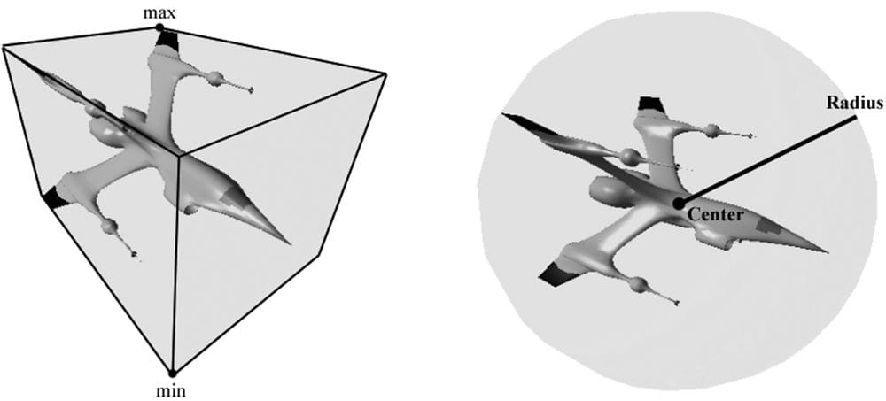
16.1.1 Drawing Instanced Data Perhaps surprisingly, we have already been drawing instanced data in all the previous chapter demos. However, the instance count has always been 1 (second parameter): cmdList->DrawIndexedInstanced(ri->IndexCount, 1, ri->StartIndexLocation, ri->BaseVertexLocation, 0); The second parameter, InstanceCount, specifies the number of times to instance the geometry we are drawing. If we specify ten, the geometry will be drawn 10 times. Drawing an object ten times alone does not really help us, though. The object will be drawn in the same place using the same materials and textures. So the next step is to figure out how to specify additional per-instance data so that we can vary the instances by rendering them with different transforms, materials, and textures. 16.1.2 Instance Data The previous version of this book obtained instance data from the input assembly stage. When creating an input layout, you can specify that data streams in per-instance rather than at a per-vertex frequency by using D3D12_INPUT_CLASSIFICATION_PER_INSTANCE_DATA instead of D3D12_INPUT_CLASSIFICATION_PER_VERTEX_DATA, respectively. You would then bind a secondary vertex buffer to the input stream that contained the instancing data. Direct3D 12 still supports this way of feeding instancing data into the pipeline, but we opt for a more modern approach. The modern approach is to create a structured buffer that contains the per-instance data for all of our instances. For example, if we were going to instance an object 100 times, we would create a structured buffer with 100 per-instance data elements. We then bind the structured buffer resource to the rendering pipeline, and index into it in the vertex shader based on the instance we are drawing. How do we know which instance is being drawn in the vertex shader? Direct3D provides the system value identifier SV_InstanceID which you can use in your vertex shader. For example, vertices of the first instance will have id 0, vertices of the second instance will have id 1, and so on. So in our vertex shader, we can index into the structured buffer to fetch the per-instance data we need. The following shader code shows how this all works: // Defaults for number of lights. #ifndef NUM_DIR_LIGHTS #define NUM_DIR_LIGHTS 3 #endif #ifndef NUM_POINT_LIGHTS #define NUM_POINT_LIGHTS 0 #endif #ifndef NUM_SPOT_LIGHTS #define NUM_SPOT_LIGHTS 0 #endif // Include structures and functions for lighting. #include "LightingUtil.hlsl" struct InstanceData { float4x4 World; float4x4 TexTransform; uint MaterialIndex; uint InstPad0; uint InstPad1; uint InstPad2; }; struct MaterialData { float4 DiffuseAlbedo; float3 FresnelR0; float Roughness; float4x4 MatTransform; uint DiffuseMapIndex; uint MatPad0; uint MatPad1; uint MatPad2; }; // An array of textures, which is only supported in shader model 5.1+. // Unlike Texture2DArray, the textures in this array can be different // sizes and formats, making it more flexible than texture arrays. Texture2D gDiffuseMap[7] : register(t0); // Put in space1, so the texture array does not overlap with these. // The texture array above will occupy registers t0, t1, …, t6 in // space0. StructuredBuffer<InstanceData> gInstanceData : register(t0, space1); StructuredBuffer<MaterialData> gMaterialData : register(t1, space1); SamplerState gsamPointWrap : register(s0); SamplerState gsamPointClamp : register(s1); SamplerState gsamLinearWrap : register(s2); SamplerState gsamLinearClamp : register(s3); SamplerState gsamAnisotropicWrap : register(s4); SamplerState gsamAnisotropicClamp : register(s5); // Constant data that varies per pass. cbuffer cbPass : register(b0) { float4x4 gView; float4x4 gInvView; float4x4 gProj; float4x4 gInvProj; float4x4 gViewProj; float4x4 gInvViewProj; float3 gEyePosW; float cbPerObjectPad1; float2 gRenderTargetSize; float2 gInvRenderTargetSize; float gNearZ; float gFarZ; float gTotalTime; float gDeltaTime; float4 gAmbientLight; // Indices [0, NUM_DIR_LIGHTS) are directional lights; // indices [NUM_DIR_LIGHTS, NUM_DIR_LIGHTS+NUM_POINT_LIGHTS) are point lights; // indices [NUM_DIR_LIGHTS+NUM_POINT_LIGHTS, // NUM_DIR_LIGHTS+NUM_POINT_LIGHT+NUM_SPOT_LIGHTS) // are spot lights for a maximum of MaxLights per object. Light gLights[MaxLights]; }; struct VertexIn { float3 PosL : POSITION; float3 NormalL : NORMAL; float2 TexC : TEXCOORD; }; struct VertexOut { float4 PosH : SV_POSITION; float3 PosW : POSITION; float3 NormalW : NORMAL; float2 TexC : TEXCOORD; // nointerpolation is used so the index is not interpolated // across the triangle. nointerpolation uint MatIndex : MATINDEX; }; VertexOut VS(VertexIn vin, uint instanceID : SV_InstanceID) { VertexOut vout = (VertexOut)0.0f; // Fetch the instance data. InstanceData instData = gInstanceData[instanceID]; float4x4 world = instData.World; float4x4 texTransform = instData.TexTransform; uint matIndex = instData.MaterialIndex; vout.MatIndex = matIndex; // Fetch the material data. MaterialData matData = gMaterialData[matIndex]; // Transform to world space. float4 posW = mul(float4(vin.PosL, 1.0f), world); vout.PosW = posW.xyz; // Assumes nonuniform scaling; otherwise, need to use inverse-transpose // of world matrix. vout.NormalW = mul(vin.NormalL, (float3x3)world); // Transform to homogeneous clip space. vout.PosH = mul(posW, gViewProj); // Output vertex attributes for interpolation across triangle. float4 texC = mul(float4(vin.TexC, 0.0f, 1.0f), texTransform); vout.TexC = mul(texC, matData.MatTransform).xy; return vout; } float4 PS(VertexOut pin) : SV_Target { // Fetch the material data. MaterialData matData = gMaterialData[pin.MatIndex]; float4 diffuseAlbedo = matData.DiffuseAlbedo; float3 fresnelR0 = matData.FresnelR0; float roughness = matData.Roughness; uint diffuseTexIndex = matData.DiffuseMapIndex; // Dynamically look up the texture in the array. diffuseAlbedo *= gDiffuseMap[diffuseTexIndex].Sample(gsamLinearWrap, pin.TexC); // Interpolating normal can unnormalize it, so renormalize it. pin.NormalW = normalize(pin.NormalW); // Vector from point being lit to eye. float3 toEyeW = normalize(gEyePosW - pin.PosW); // Light terms. float4 ambient = gAmbientLight*diffuseAlbedo; Material mat = { diffuseAlbedo, fresnelR0, roughness }; float4 directLight = ComputeDirectLighting(gLights, mat, pin.PosW, pin.NormalW, toEyeW); float4 litColor = ambient + directLight; // Common convention to take alpha from diffuse albedo. litColor.a = diffuseAlbedo.a; return litColor; } Note that we no longer have a per-object constant buffer. The per-object data comes from the instance buffer. Observe also how we use dynamic indexing to associate a different material for each instance, and a different texture. We are able to get quite a lot of per-instance variety in a single draw call! For completeness, the corresponding root signature description is shown below that corresponds to the above shader programs: CD3DX12_DESCRIPTOR_RANGE texTable; texTable.Init(D3D12_DESCRIPTOR_RANGE_TYPE_SRV, 7, 0, 0); // Root parameter can be a table, root descriptor or root constants. CD3DX12_ROOT_PARAMETER slotRootParameter[4]; // Perfomance TIP: Order from most frequent to least frequent. slotRootParameter[0].InitAsShaderResourceView(0, 1); slotRootParameter[1].InitAsShaderResourceView(1, 1); slotRootParameter[2].InitAsConstantBufferView(0); slotRootParameter[3].InitAsDescriptorTable(1, &texTable, D3D12_SHADER_VISIBILITY_PIXEL); auto staticSamplers = GetStaticSamplers(); // A root signature is an array of root parameters. CD3DX12_ROOT_SIGNATURE_DESC rootSigDesc(4, slotRootParameter, (UINT)staticSamplers.size(), staticSamplers.data(), D3D12_ROOT_SIGNATURE_FLAG_ALLOW_INPUT_ASSEMBLER_INPUT_LAYOUT); As in the last chapter, we bind all the scene materials and textures once per-frame, and the only per draw call resource we need to set is the structured buffer with the instanced data: void InstancingAndCullingApp::Draw(const GameTimer& gt) { … // Bind all the materials used in this scene. For structured buffers, we // can bypass the heap and set as a root descriptor. auto matBuffer = mCurrFrameResource->MaterialBuffer->Resource(); mCommandList->SetGraphicsRootShaderResourceView(1, matBuffer->GetGPUVirtualAddress()); auto passCB = mCurrFrameResource->PassCB->Resource(); mCommandList->SetGraphicsRootConstantBufferView(2, passCB->GetGPUVirtualAddress()); // Bind all the textures used in this scene. mCommandList->SetGraphicsRootDescriptorTable(3, mSrvDescriptorHeap->GetGPUDescriptorHandleForHeapStart()); DrawRenderItems(mCommandList.Get(), mOpaqueRitems); … } void InstancingAndCullingApp::DrawRenderItems( ID3D12GraphicsCommandList* cmdList, const std::vector<RenderItem*>& ritems) { // For each render item… for(size_t i = 0; i < ritems.size(); ++i) { auto ri = ritems[i]; cmdList->IASetVertexBuffers(0, 1, &ri->Geo->VertexBufferView()); cmdList->IASetIndexBuffer(&ri->Geo->IndexBufferView()); cmdList->IASetPrimitiveTopology(ri->PrimitiveType); // Set the instance buffer to use for this render-item. // For structured buffers, we can bypass // the heap and set as a root descriptor. auto instanceBuffer = mCurrFrameResource->InstanceBuffer->Resource(); mCommandList->SetGraphicsRootShaderResourceView( 0, instanceBuffer->GetGPUVirtualAddress()); cmdList->DrawIndexedInstanced(ri->IndexCount, ri->InstanceCount, ri->StartIndexLocation, ri->BaseVertexLocation, 0); } } 16.1.3 Creating the Instanced Buffer The instance buffer stores the data that varies per-instance. It looks a lot like the data we previously put in our per-object constant buffer. On the CPU side, our instance data structure looks like this: struct InstanceData { DirectX::XMFLOAT4X4 World = MathHelper::Identity4x4(); DirectX::XMFLOAT4X4 TexTransform = MathHelper::Identity4x4(); UINT MaterialIndex; UINT InstancePad0; UINT InstancePad1; UINT InstancePad2; }; The per-instance data in system memory is stored as part of the render-item structure, as the render-item maintains how many times it should be instanced: struct RenderItem { … std::vector<InstanceData> Instances; … }; For the GPU to consume the instance data, we need to create a structured buffer with element type InstanceData. Moreover, this buffer will be dynamic (i.e., an upload buffer) so that we can update it every frame; in our demo, we copy the instanced data of only the visible instances into the structure buffer (this is related to frustum culling, see §16.3), and the set of visible instances will change as the camera moves/looks around. Creating a dynamic buffer is simple with our UploadBuffer helper class: struct FrameResource { public: FrameResource(ID3D12Device* device, UINT passCount, UINT maxInstanceCount, UINT materialCount); FrameResource(const FrameResource& rhs) = delete; FrameResource& operator=(const FrameResource& rhs) = delete; ˜FrameResource(); // We cannot reset the allocator until the GPU is done processing the commands. // So each frame needs their own allocator. Microsoft::WRL::ComPtr<ID3D12CommandAllocator> CmdListAlloc; // We cannot update a cbuffer until the GPU is done processing the commands // that reference it. So each frame needs their own cbuffers. // std::unique_ptr<UploadBuffer<FrameConstants>> FrameCB = nullptr; std::unique_ptr<UploadBuffer<PassConstants>> PassCB = nullptr; std::unique_ptr<UploadBuffer<MaterialData>> MaterialBuffer = nullptr; // NOTE: In this demo, we instance only one render-item, so we only have // one structured buffer to store instancing data. To make this more // general (i.e., to support instancing multiple render-items), you // would need to have a structured buffer for each render-item, and // allocate each buffer with enough room for the maximum number of // instances you would ever draw. This sounds like a lot, but it is // actually no more than the amount of per-object constant data we // would need if we were not using instancing. For example, if we // were drawing 1000 objects without instancing, we would create a // constant buffer with enough room for a 1000 objects. With instancing, // we would just create a structured buffer large enough to store the // instance data for 1000 instances. std::unique_ptr<UploadBuffer<InstanceData>> InstanceBuffer = nullptr; // Fence value to mark commands up to this fence point. This lets us // check if these frame resources are still in use by the GPU. UINT64 Fence = 0; }; FrameResource::FrameResource(ID3D12Device* device, UINT passCount, UINT maxInstanceCount, UINT materialCount) { ThrowIfFailed(device->CreateCommandAllocator( D3D12_COMMAND_LIST_TYPE_DIRECT, IID_PPV_ARGS(CmdListAlloc.GetAddressOf()))); PassCB = std::make_unique<UploadBuffer<PassConstants>>( device, passCount, true); MaterialBuffer = std::make_unique<UploadBuffer<MaterialData>>( device, materialCount, false); InstanceBuffer = std::make_unique<UploadBuffer<InstanceData>>( device, maxInstanceCount, false); } Note that InstanceBuffer is not a constant buffer, so we specify false for the last parameter. 16.2 BOUNDING VOLUMES AND FRUSTUMS In order to implement frustum culling, we need to become familiar with the mathematical representation of a frustum and various bounding volumes. Bounding volumes are primitive geometric objects that approximate the volume of an object—see Figure 16.1. The tradeoff is that although the bounding volume only approximates the object its form has a simple mathematical representation, which makes it easy to work with.
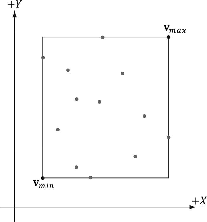
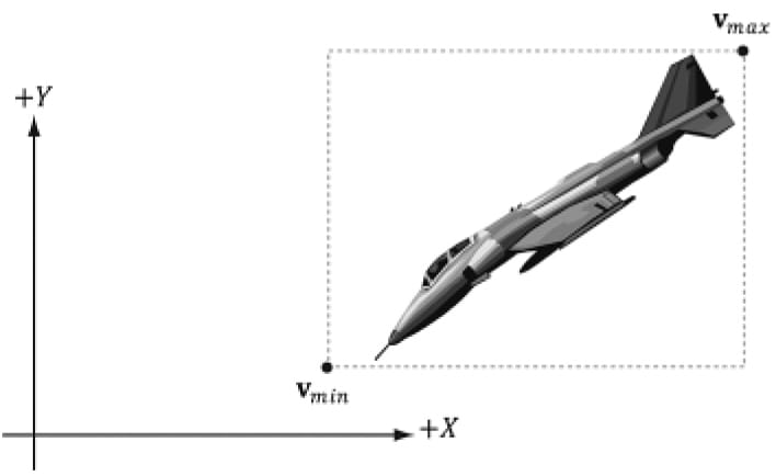
Figure 16.1. A mesh rendered with its AABB and bounding sphere. 16.2.1 DirectX Math Collision We use the DirectXCollision.h utility library, which is part of DirectX Math. This library provides fast implementations to common geometric primitive intersection tests such as ray/triangle intersection, ray/box intersection, box/box intersection, box/plane intersection, box/frustum, sphere/frustum, and much more. Exercise 3 asks you to explore this library to get familiar with what it offers. 16.2.2 Boxes The axis-aligned bounding box (AABB) of a mesh is a box that tightly surrounds the mesh and such that its faces are parallel to the major axes. An AABB can be described by a minimum point vmin and a maximum point vmax(see Figure 16.2). The minimum point vmin is found by searching through all the vertices of the mesh and finding the minimum x-, y-, and z-coordinates, and the maximum point vmax is found by searching through all the vertices of the mesh and finding the maximum x-, y-, and z-coordinates.
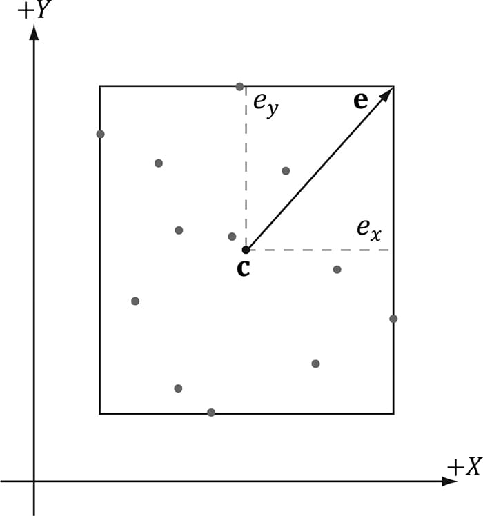
Figure 16.2. The AABB of a set of points using minimum and maximum point representation. Alternatively, an AABB can be represented with the box center point c and extents vector e, which stores the distance from the center point to the sides of the box along the coordinate axes (see Figure 16.3).
Figure 16.3. The AABB of a set of points using center and extents representation. The DirectX collision library uses the center/extents representation: struct BoundingBox { static const size_t CORNER_COUNT = 8; XMFLOAT3 Center; // Center of the box. XMFLOAT3 Extents; // Distance from the center to each side. … It is easy to convert from one representation to the other. For example, given a bounding box defined by vmin and vmax, the center/extents representation is given by:
The following code shows how we compute the bounding box of the skull mesh in this chapter’s demo: XMFLOAT3 vMinf3(+MathHelper::Infinity, +MathHelper::Infinity, +MathHelper::Infinity); XMFLOAT3 vMaxf3(-MathHelper::Infinity, -MathHelper::Infinity, -MathHelper::Infinity); XMVECTOR vMin = XMLoadFloat3(&vMinf3); XMVECTOR vMax = XMLoadFloat3(&vMaxf3); std::vector<Vertex> vertices(vcount); for(UINT i = 0; i < vcount; ++i) { fin >> vertices[i].Pos.x >> vertices[i].Pos.y >> vertices[i].Pos.z; fin >> vertices[i].Normal.x >> vertices[i].Normal.y >> vertices[i].Normal.z; XMVECTOR P = XMLoadFloat3(&vertices[i].Pos); // Project point onto unit sphere and generate spherical texture coordinates. XMFLOAT3 spherePos; XMStoreFloat3(&spherePos, XMVector3Normalize(P)); float theta = atan2f(spherePos.z, spherePos.x); // Put in [0, 2pi]. if(theta < 0.0f) theta += XM_2PI; float phi = acosf(spherePos.y); float u = theta / (2.0f*XM_PI); float v = phi / XM_PI; vertices[i].TexC = { u, v }; vMin = XMVectorMin(vMin, P); vMax = XMVectorMax(vMax, P); } BoundingBox bounds; XMStoreFloat3(&bounds.Center, 0.5f*(vMin + vMax)); XMStoreFloat3(&bounds.Extents, 0.5f*(vMax - vMin)); The XMVectorMin and XMVectorMax functions return the vectors:
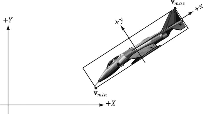
16.2.2.1 Rotations and Axis-Aligned Bounding Boxes Figure 16.4 shows that a box axis-aligned in one coordinate system may not be axis-aligned with a different coordinate system. In particular, if we compute the AABB of a mesh in local space, it gets transformed to an oriented bounding box (OBB) in world space. However, we can always transform into the local space of the mesh and do the intersection there where the box is axis-aligned.
Figure 16.4. The bounding box is axis aligned with the xy-frame, but not with the XY-frame. Alternatively, we can recompute the AABB in the world space, but this can result in a “fatter” box that is a poorer approximation to the actual volume (see Figure 16.5).
Figure 16.5. The bounding box is axis aligned with the XY-frame. Yet another alternative is to abandon axis-aligned bounding boxes, and just work with oriented bounding boxes, where we maintain the orientation of the box relative to the world space. The DirectX collision library provides the following structure for representing an oriented bounding box. struct BoundingOrientedBox { static const size_t CORNER_COUNT = 8; XMFLOAT3 Center; // Center of the box. XMFLOAT3 Extents; // Distance from the center to each side. XMFLOAT4 Orientation; // Unit quaternion representing rotation (box -> world). …
An AABB and OBB can also be constructed from a set of points using the DirectX collision library with the following static member functions: void BoundingBox::CreateFromPoints( _Out_ BoundingBox& Out, _In_ size_t Count, _In_reads_bytes_(sizeof(XMFLOAT3)+Stride*(Count-1)) const XMFLOAT3* pPoints, _In_ size_t Stride ); void BoundingOrientedBox::CreateFromPoints( _Out_ BoundingOrientedBox& Out, _In_ size_t Count, _In_reads_bytes_(sizeof(XMFLOAT3)+Stride*(Count-1)) const XMFLOAT3* pPoints, _In_ size_t Stride ); If your vertex structure looks like this: struct Basic32 { XMFLOAT3 Pos; XMFLOAT3 Normal; XMFLOAT2 TexC; }; And you have an array of vertices forming your mesh: std::vector<Vertex::Basic32> vertices; Then you call this function like so: BoundingBox box; BoundingBox::CreateFromPoints( box, vertices.size(), &vertices[0].Pos, sizeof(Vertex::Basic32)); The stride indicates how many bytes to skip to get to the next position element.
16.2.3 Spheres The bounding sphere of a mesh is a sphere that tightly surrounds the mesh. A bounding sphere can be described with a center point and radius. One way to compute the bounding sphere of a mesh is to first compute its AABB. We then take the center of the AABB as the center of the bounding sphere:
The radius is then taken to be the maximum distance between any vertex p in the mesh from the center c:
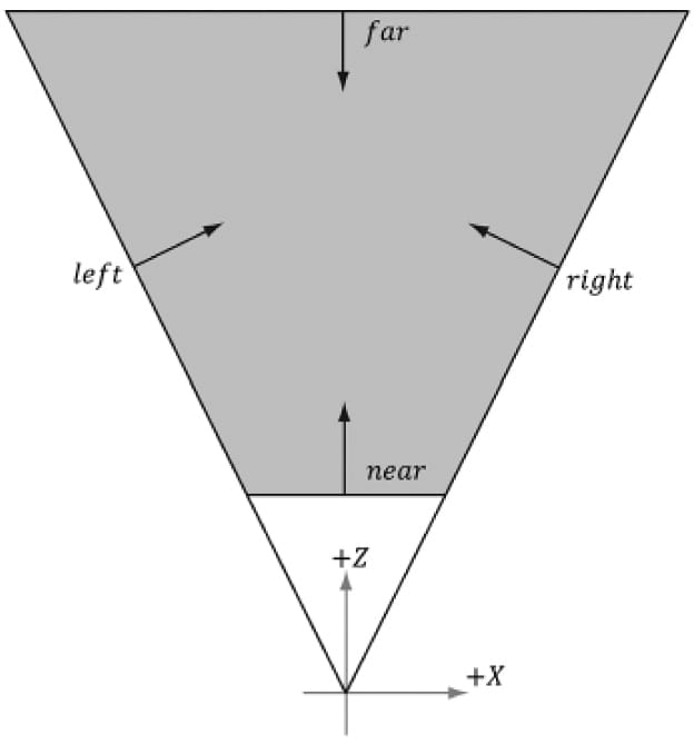
Suppose we compute the bounding sphere of a mesh in local space. After the world transform, the bounding sphere may not tightly surround the mesh due to scaling. Thus the radius needs to be rescaled accordingly. To compensate for non-uniform scaling, we must scale the radius by the largest scaling component so that the sphere encapsulates the transformed mesh. Another possible strategy is to avoid scaling all together by having all your meshes modeled to the same scale of the game world. This way, models will not need to be rescaled once loaded into the application. The DirectX collision library provides the following structure for representing a bounding sphere: struct BoundingSphere { XMFLOAT3 Center; // Center of the sphere. float Radius; // Radius of the sphere. … And it provides the following static member function for creating one from a set of points: void BoundingSphere::CreateFromPoints( _Out_ BoundingSphere& Out, _In_ size_t Count, _In_reads_bytes_(sizeof(XMFLOAT3)+Stride*(Count-1)) const XMFLOAT3* pPoints, _In_ size_t Stride ); 16.2.4 Frustums We are well familiar with frustums from Chapter 5. One way to specify a frustum mathematically is as the intersection of six planes: the left/right planes, the top/bottom planes, and the near/far planes. We assume the six frustum planes are “inward” facing—see Figure 16.6.
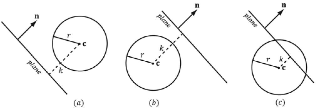
Figure 16.6. The intersection of the positive half spaces of the frustum planes defines the frustum volume. This six plane representation makes it easy to do frustum and bounding volume intersection tests. 16.2.4.1 Constructing the Frustum Planes One easy way to construct the frustum planes is in view space, where the frustum takes on a canonical form centered at the origin looking down the positive z-axis. Here, the near and far planes are trivially specified by their distances along the z-axis, the left and right planes are symmetric and pass through the origin (see Figure 16.6 again), and the top and bottom planes are symmetric and pass through the origin. Consequently, we do not even need to store the full plane equations to represent the frustum in view space, we just need the plane slopes for the top/bottom/left/right planes, and the z distances for the near and far plane. The DirectX collision library provides the following structure for representing a frustum: struct BoundingFrustum { static const size_t CORNER_COUNT = 8; XMFLOAT3 Origin; // Origin of the frustum (and projection). XMFLOAT4 Orientation; // Quaternion representing rotation. float RightSlope; // Positive X slope (X/Z). float LeftSlope; // Negative X slope. float TopSlope; // Positive Y slope (Y/Z). float BottomSlope; // Negative Y slope. float Near, Far; // Z of the near plane and far plane. … In the local space of the frustum (e.g., view space for the camera), the Origin would be zero, and the Orientation would represent an identity transform (no rotation). We can position and orientate the frustum somewhere in the world by specifying an Origin position and Orientation quaternion. If we cached the frustum vertical field of view, aspect ratio, near and far planes of our camera, then we can determine the frustum plane equations in view space with a little mathematical effort. However, it is also possible to derive the frustum plane equations in view space from the projection matrix in a number of ways (see [Lengyel02] or [Möller08] for two different ways). The XNA collision library takes the following strategy. In NDC space, the view frustum has been warped into the box [−1,1] × [−1,1] × [0,1]. So the eight corners of the view frustum are simply: // Corners of the projection frustum in homogenous space. static XMVECTORF32 HomogenousPoints[6] = { { 1.0f, 0.0f, 1.0f, 1.0f }, // right (at far plane) { -1.0f, 0.0f, 1.0f, 1.0f }, // left { 0.0f, 1.0f, 1.0f, 1.0f }, // top { 0.0f, -1.0f, 1.0f, 1.0f }, // bottom { 0.0f, 0.0f, 0.0f, 1.0f }, // near { 0.0f, 0.0f, 1.0f, 1.0f } // far }; We can compute the inverse of the projection matrix (as well is invert the homogeneous divide), to transform the eight corners from NDC space back to view space. One we have the eight corners of the frustum in view space, some simple mathematics is used to compute the plane equations (again, this is simple because in view space, the frustum is positioned at the origin, and axis aligned). The following DirectX collision code computes the frustum in view space from a projection matrix: //---------------------------------------------------------------------------- // Build a frustum from a persepective projection matrix. The matrix may only // contain a projection; any rotation, translation or scale will cause the // constructed frustum to be incorrect. //---------------------------------------------------------------------------- _Use_decl_annotations_ inline void XM_CALLCONV BoundingFrustum::CreateFromMatrix( BoundingFrustum& Out, FXMMATRIX Projection ) { // Corners of the projection frustum in homogenous space. static XMVECTORF32 HomogenousPoints[6] = { { 1.0f, 0.0f, 1.0f, 1.0f }, // right (at far plane) { -1.0f, 0.0f, 1.0f, 1.0f }, // left { 0.0f, 1.0f, 1.0f, 1.0f }, // top { 0.0f, -1.0f, 1.0f, 1.0f }, // bottom { 0.0f, 0.0f, 0.0f, 1.0f }, // near { 0.0f, 0.0f, 1.0f, 1.0f } // far }; XMVECTOR Determinant; XMMATRIX matInverse = XMMatrixInverse( &Determinant, Projection ); // Compute the frustum corners in world space. XMVECTOR Points[6]; for( size_t i = 0; i < 6; ++i ) { // Transform point. Points[i] = XMVector4Transform( HomogenousPoints[i], matInverse ); } Out.Origin = XMFLOAT3( 0.0f, 0.0f, 0.0f ); Out.Orientation = XMFLOAT4( 0.0f, 0.0f, 0.0f, 1.0f ); // Compute the slopes. Points[0] = Points[0] * XMVectorReciprocal( XMVectorSplatZ( Points[0] ) ); Points[1] = Points[1] * XMVectorReciprocal( XMVectorSplatZ( Points[1] ) ); Points[2] = Points[2] * XMVectorReciprocal( XMVectorSplatZ( Points[2] ) ); Points[3] = Points[3] * XMVectorReciprocal( XMVectorSplatZ( Points[3] ) ); Out.RightSlope = XMVectorGetX( Points[0] ); Out.LeftSlope = XMVectorGetX( Points[1] ); Out.TopSlope = XMVectorGetY( Points[2] ); Out.BottomSlope = XMVectorGetY( Points[3] ); // Compute near and far. Points[4] = Points[4] * XMVectorReciprocal( XMVectorSplatW( Points[4] ) ); Points[5] = Points[5] * XMVectorReciprocal( XMVectorSplatW( Points[5] ) ); Out.Near = XMVectorGetZ( Points[4] ); Out.Far = XMVectorGetZ( Points[5] ); } 16.2.4.2 Frustum/Sphere Intersection For frustum culling, one test we will want to perform is a frustum/sphere intersection test. This tells us whether a sphere intersects the frustum. Note that a sphere completely inside the frustum counts as an intersection because we treat the frustum as a volume, not just a boundary. Because we model a frustum as six inward facing planes, a frustum/sphere test can be stated as follows: If there exists a frustum plane L such that the sphere is in the negative half-space of L, then we can conclude that the sphere is completely outside the frustum. If such a plane does not exist, then we conclude that the sphere intersects the frustum. So a frustum/sphere intersection test reduces to six sphere/plane tests. Figure 16.7 shows the setup of a sphere/plane intersection test. Let the sphere have center point c and radius r. Then the signed distance from the center of the sphere to the plane is k = n · c + d(Appendix C). If |k| ≤ r then the sphere intersects the plane. If k < −r then the sphere is behind the plane. If k > r then the sphere is in front of the plane and the sphere intersects the positive half-space of the plane. For the purposes of the frustum/sphere intersection test, if the sphere is in front of the plane, then we count it as an intersection because it intersects the positive half-space the plane defines.
Figure 16.7. Sphere/plane intersection. (a) k > r and the sphere intersects the positive half-space of the plane. (b) k < −r and the sphere is completely behind the plane in the negative half-space. (c) |k| ≤ r and the sphere intersects the plane. The BoundingFrustum class provides the following member function to test if a sphere intersects a frustum. Note that the sphere and frustum must be in the same coordinate system for the test to make sense. enum ContainmentType { // The object is completely outside the frustum. DISJOINT = 0, // The object intersects the frustum boundaries. INTERSECTS = 1, // The object lies completely inside the frustum volume. CONTAINS = 2, }; ContainmentType BoundingFrustum::Contains( _In_ const BoundingSphere& sphere ) const;
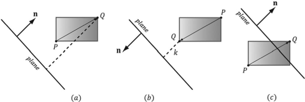
ContainmentType BoundingSphere::Contains( _In_ const BoundingFrustum& fr ) const; 16.2.4.3 Frustum/AABB Intersection The frustum/AABB intersection test follows the same strategy as the frustum/sphere test. Because we model a frustum as six inward facing planes, a frustum/AABB test can be stated as follows: If there exists a frustum plane L such that the box is in the negative half-space of L, then we can conclude that the box is completely outside the frustum. If such a plane does not exist, then we conclude that the box intersects the frustum. So a frustum/AABB intersection test reduces to six AABB/plane tests. The algorithm for an AABB/plane test is as follows. Find the box diagonal vector v = , passing through the center of the box, that is most aligned with the plane normal n. From Figure 16.8, (a) if P is in front of the plane, then Q must be also in front of the plane; (b) if Q is behind the plane, then P must be also be behind the plane; (c) if P is behind the plane and Q is in front of the plane, then the box intersects the plane.
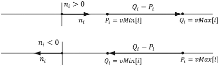
Figure 16.8. AABB/plane intersection test. The diagonal is always the diagonal most directed with the plane normal. Finding PQ most aligned with the plane normal vector n can be done with the following code: // For each coordinate axis x, y, z… for(int j = 0; j < 3; ++j) { // Make PQ point in the same direction as // the plane normal on this axis. if( planeNormal[j] >= 0.0f ) { P[j] = box.minPt[j]; Q[j] = box.maxPt[j]; } else { P[j] = box.maxPt[j]; Q[j] = box.minPt[j]; } } This code just looks at one dimension at a time, and chooses Pi and Qi such that Qi − Pi has the same sign as the plane normal coordinate ni (Figure 16.9).
Figure 16.9. (Top) The normal component along the ith axis is positive, so we choose Pi = vMin[i] and Qi = vMax[i] so that Qi − Pi has the same sign as the plane normal coordinate ni. (Bottom) The normal component along the ith axis is negative, so we choose Pi = vMax[i] and Qi = vMin[i] so that Qi − Pi has the same sign as the plane normal coordinate ni. The BoundingFrustum class provides the following member function to test if an AABB intersects a frustum. Note that the AABB and frustum must be in the same coordinate system for the test to make sense. ContainmentType BoundingFrustum::Contains( _In_ const BoundingBox& box ) const;
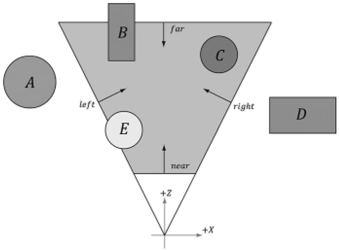
16.3 FRUSTUM CULLING Recall from Chapter 5 that the hardware automatically discards triangles that are outside the viewing frustum in the clipping stage. However, if we have millions of triangles, all the triangles are still submitted to the rendering pipeline via draw calls (which has API overhead), and all the triangles go through the vertex shader, possibly through the tessellation stages, and possibly through the geometry shader, only to be discarded during the clipping stage. Clearly, this is wasteful inefficiency. The idea of frustum culling is for the application code to cull groups of triangles at a higher level than on a per-triangle basis. Figure 16.10 shows a simple example. We build a bounding volume, such as a sphere or box, around each object in the scene. If the bounding volume does not intersect the frustum, then we do not need to submit the object (which could contain thousands of triangles) to Direct3D for drawing. This saves the GPU from having to do wasteful computations on invisible geometry, at the cost of an inexpensive CPU test. Assuming a camera with a 90° field of view and infinitely far away far plane, the camera frustum only occupies 1/6th of the world volume, so 5/6thof the world objects can be frustum culled, assuming objects are evenly distributed throughout the scene. In practice, cameras use smaller field of view angles than 90° and a finite far plane, which means we could cull even more than 5/6th of the scene objects.
Figure 16.10. The objects bounded by volumes A and D are completely outside the frustum, and so do not need to be drawn. The object corresponding to volume C is completely inside the frustum, and needs to be drawn. The objects bounded by volumes B and E are partially outside the frustum and partially inside the frustum; we must draw these objects and let the hardware clip and triangles outside the frustum.
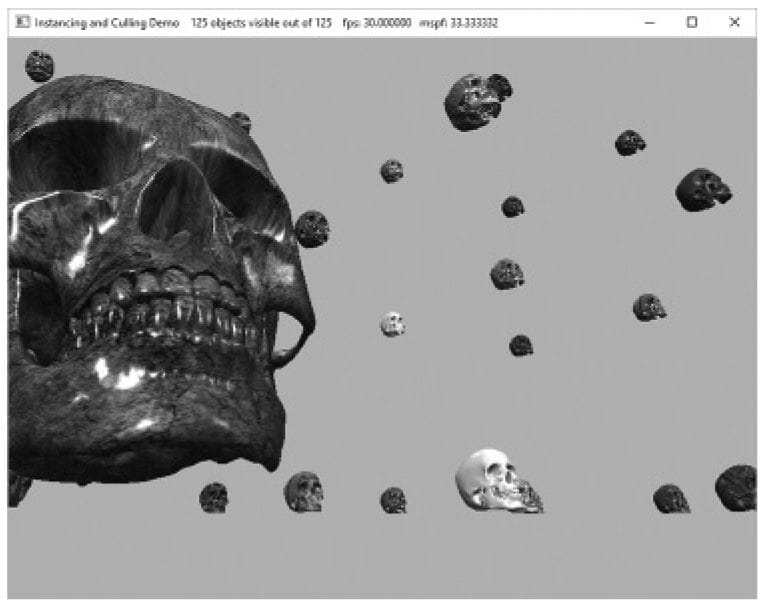
Figure 16.11. Screenshot of the “Instancing and Culling” demo. In our demo, we render a 5 × 5 × 5 grid of skull meshes (see Figure 16.11) using instancing. We compute the AABB of the skull mesh in local space. In the UpdateInstanceData method, we perform frustum culling on all of our instances. If the instance intersects the frustum, then we add it to the next available slot in our structured buffer containing the instance data and increment the visibleInstanceCount counter. This way, the front of the structured buffer contains the data for all the visible instances. (Of course, the structured buffer is sized to match the number of instances in case all the instances are visible.) Because the AABB of the skull mesh is in local space, we must transform the view frustum into the local space of each instance in order to perform the intersection test; we could use alternative spaces, like transform the AABB to world space and the frustum to world space, for example. The frustum culling update code is given below: XMMATRIX view = mCamera.GetView(); XMMATRIX invView = XMMatrixInverse(&XMMatrixDeterminant(view), view); auto currInstanceBuffer = mCurrFrameResource->InstanceBuffer.get(); for(auto& e : mAllRitems) { const auto& instanceData = e->Instances; int visibleInstanceCount = 0; for(UINT i = 0; i < (UINT)instanceData.size(); ++i) { XMMATRIX world = XMLoadFloat4x4(&instanceData[i].World); XMMATRIX texTransform = XMLoadFloat4x4(&instanceData[i].TexTransform); XMMATRIX invWorld = XMMatrixInverse(&XMMatrixDeterminant(world), world); // View space to the object’s local space. XMMATRIX viewToLocal = XMMatrixMultiply(invView, invWorld); // Transform the camera frustum from view space to the object’s local space. BoundingFrustum localSpaceFrustum; mCamFrustum.Transform(localSpaceFrustum, viewToLocal); // Perform the box/frustum intersection test in local space. if(localSpaceFrustum.Contains(e->Bounds) != DirectX::DISJOINT) { InstanceData data; XMStoreFloat4x4(&data.World, XMMatrixTranspose(world)); XMStoreFloat4x4(&data.TexTransform, XMMatrixTranspose(texTransform)); data.MaterialIndex = instanceData[i].MaterialIndex; // Write the instance data to structured buffer for the visible objects. currInstanceBuffer->CopyData(visibleInstanceCount++, data); } } e->InstanceCount = visibleInstanceCount; // For informational purposes, output the number of instances // visible over the total number of instances. std::wostringstream outs; outs.precision(6); outs << L"Instancing and Culling Demo" << L" " << e->InstanceCount << L" objects visible out of " << e->Instances.size(); mMainWndCaption = outs.str(); } Even though our instanced buffer has room for every instance, we only draw the visible instances which correspond to instances from 0 to visibleInstanceCount-1: cmdList->DrawIndexedInstanced(ri->IndexCount, ri->InstanceCount, ri->StartIndexLocation, ri->BaseVertexLocation, 0); Figure 16.12 shows the performance difference between having frustum culling enabled and not. With frustum culling, we only submit eleven instances to the rendering pipeline for processing. Without frustum culling, we submit all 125 instances to the rendering pipeline for processing. Even though the visible scene is the same, with frustum culling disabled, we waste computation power drawing over a 100 skull meshes whose geometry is eventually discarded during the clipping stage. Each skull has about 60K triangles, so that is a lot of vertices to process and a lot of triangles to clip per skull. By doing one frustum/AABB test, we can reject 60K triangles from even being sent to the graphics pipeline—this is the advantage of frustum culling and we see the difference in the frames per second.
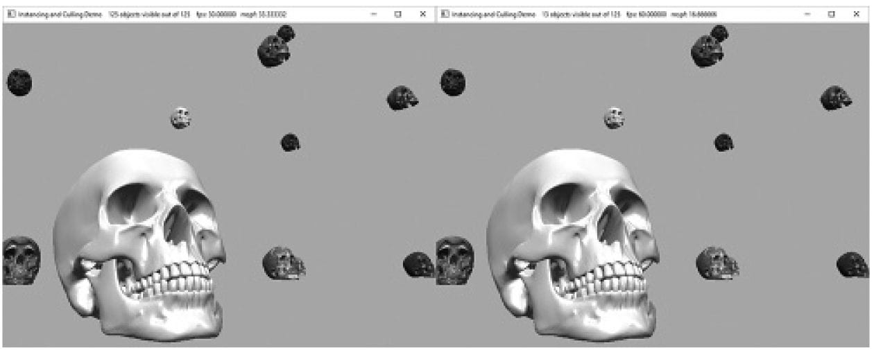
Figure 16.12. (Left) Frustum culling is turned off, and we are rendering all 125 instances, and it takes about 33.33 ms to render a frame (Right) Frustum culling is turned on, and we see that 13 out of 125 instances are visible, and our frame rate doubles. 16.4 SUMMARY 1. Instancing refers to drawing the same object more than once in a scene, but with different positions, orientations, scales, materials, and textures. To save memory, we can only create one mesh, and submit multiple draw calls to Direct3D with a different world matrix, material, and texture. To avoid the API overhead of issuing resource changes and multiple draw calls, we can bind an SRV to a structured buffer that contains all of our instance data and index into it in our vertex shader using the SV_InstancedID value. Furthermore, we can use dynamic indexing to index into arrays of textures. The number of instances to draw with one draw call is specified by the second parameter, InstanceCount, of the ID3D12GraphicsCommandList::DrawIndexedInstanced method. 2. Bounding volumes are primitive geometric objects that approximate the volume of an object. The tradeoff is that although the bounding volume only approximates the object its form has a simple mathematical representation, which makes it easy to work with. Examples of bounding volumes are spheres, axis-aligned bounding boxes (AABB), and oriented bounding boxes (OBB). The DirectXCollision.h library has structures representing bounding volumes, and functions for transforming them, and computing various intersection tests. 3. The GPU automatically discards triangles that are outside the viewing frustum in the clipping stage. However, clipped triangles are still submitted to the rendering pipeline via draw calls (which has API overhead), and all the triangles go through the vertex shader, possibly through the tessellation stages, and possibly through the geometry shader, only to be discarded during the clipping stage. To fix this inefficiency, we can implement frustum culling. The idea is to build a bounding volume, such as a sphere or box, around each object in the scene. If the bounding volume does not intersect the frustum, then we do not need to submit the object (which could contain thousands of triangles) to Direct3D for drawing. This saves the GPU from having to do wasteful computations on invisible geometry, at the cost of an inexpensive CPU test. 16.5 EXERCISES 1. Modify the “Instancing and Culling” demo to use bounding spheres instead of bounding boxes. 2. The plane equations in NDC space take on a very simple form. All points inside the view frustum are bounded as follows:
In particular, the left plane equation is given by x = −1 and the right plane equation is given by x = 1 in NDC space. In homogeneous clip space before the perspective divide, all points inside the view frustum are bounded as follows:
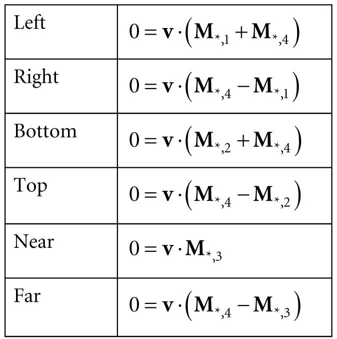
Here, the left plane is defined by w = −x and the right plane is defined by w = x. Let M = VP be the view-projection matrix product, and let v = (x, y, z, 1) be a point in world space inside the frustum. Consider to show that the inward facing frustum planes in world space are given by:
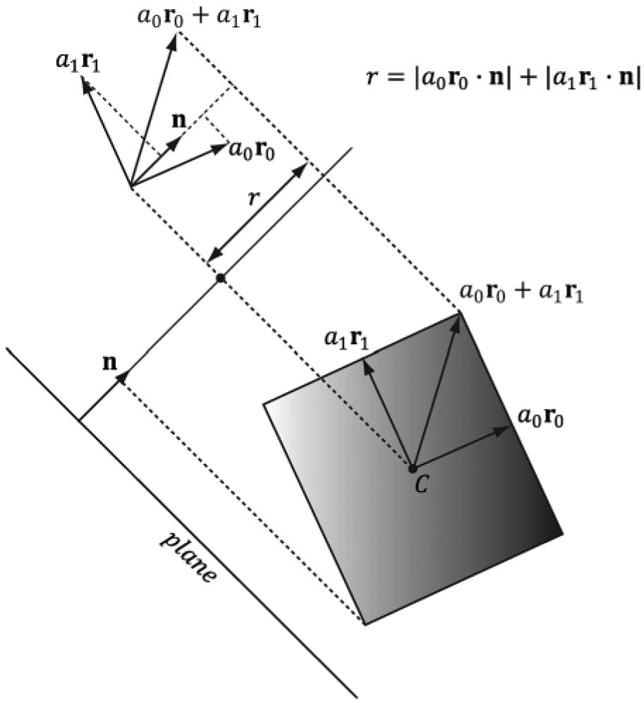
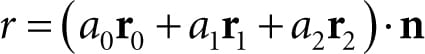
3. Examine the DirectXCollision.h header file to get familiar with the functions it provides for intersection tests and bounding volume transformations. 4. An OBB can be defined by a center point C, three orthonormal axis vectors r0, r1, and r2 defining the box orientation, and three extent lengths a0, a1, and a2 along the box axes r0, r1, and r2, respectively, that give the distance from the box center to the box sides. 1. Consider Figure 16.13 (which shows the situation in 2D) and conclude the projected “shadow” of the OBB onto the axis defined by the normal vector is 2r, where
Figure 16.13. Plane/OBB intersection setup 2. In the previous formula for r, explain why we must take the absolute values instead of just computing ? 3. Derive a plane/OBB intersection test that determines if the OBB is in front of the plane, behind the plane, or intersecting the plane. 4. An AABB is a special case of an OBB, so this test also works for an AABB. However, the formula for r simplifies in the case of an AABB. Find the simplified formula for r for the AABB case. All materials on the site are licensed Creative Commons Attribution-Sharealike 3.0 Unported CC BY-SA 3.0 & GNU Free Documentation License (GFDL) If you are the copyright holder of any material contained on our site and intend to remove it, please contact our site administrator for approval. © 2016-2026 All site design rights belong to S.Y.A. |