Introduction to 3D Game Programming with DirectX 12 (Computer Science) (2016)

Part 3

TOPICS

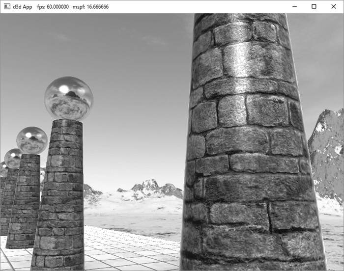
In Chapter 9, we introduced texture mapping, which enabled us to map fine details from an image onto our triangles. However, our normal vectors are still defined at the coarser vertex level and interpolated over the triangle. For part of this chapter, we study a popular method for specifying surface normals at a higher resolution. Specifying surface normals at a higher resolution increases the detail of the lighting, but the mesh geometry detail remains unchanged.

Objectives:

1. To understand why we need normal mapping.

2. To discover how normal maps are stored.

3. To learn how normal maps can be created.

4. To find out the coordinate system the normal vectors in normal maps are stored relative to and how it relates to the object space coordinate system of a 3D triangle.

5. To learn how to implement normal mapping in a vertex and pixel shader.

19.1 MOTIVATION

Consider Figure 19.1 from the Cube Mapping demo of the preceding chapter. The specular highlights on the cone shaped columns do not look right—they look unnaturally smooth compared to the bumpiness of the brick texture. This is because the underlying mesh geometry is smooth, and we have merely applied the image of bumpy bricks over the smooth cylindrical surface. However, the lighting calculations are performed based on the mesh geometry (in particular, the interpolated vertex normals), and not the texture image. Thus the lighting is not completely consistent with the texture.

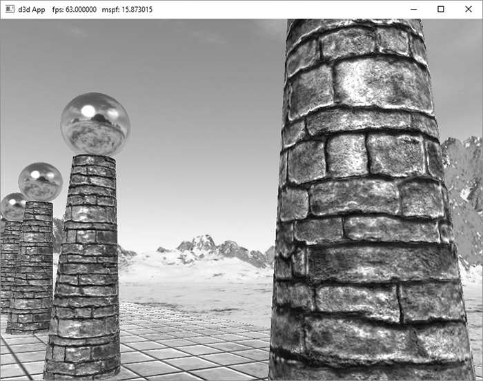
Figure 19.1. Smooth specular highlights.

Ideally, we would tessellate the mesh geometry so much that the actual bumps and crevices of the bricks could be modeled by the underlying geometry. Then the lighting and texture could be made consistent. Hardware tessellation could help in this area, but we still need a way to specify the normals for the vertices generated by the tessellator (using interpolated normals does not increase our normal resolution).

Another possible solution would be to bake the lighting details directly into the textures. However, this will not work if the lights are allowed to move, as the texel colors will remain fixed as the lights move.

Thus our goal is to find a way to implement dynamic lighting such that the fine details that show up in the texture map also show up in the lighting. Since textures provide us with the fine details to begin with, it is natural to look for a texture mapping solution to this problem. Figure 19.2 shows the same scene shown in Figure 19.1 with normal mapping; we can see now that the dynamic lighting is much more consistent with the brick texture.

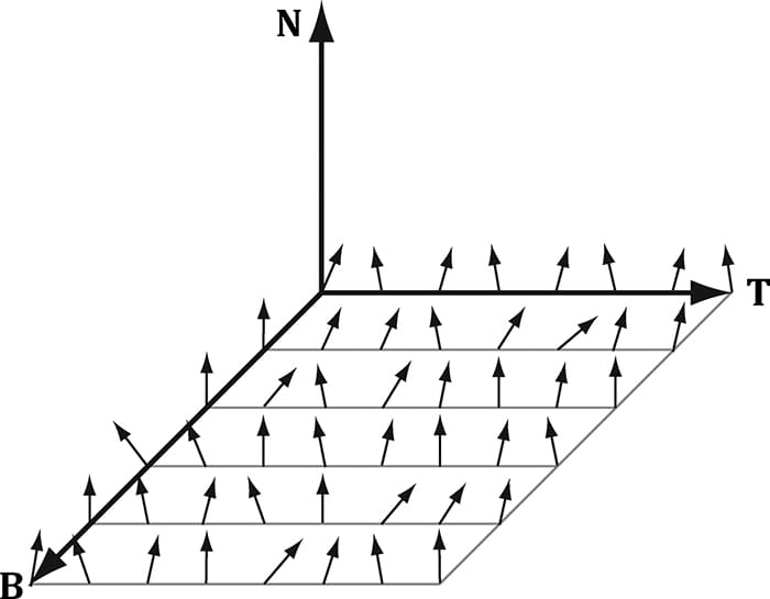
Figure 19.2. Bumpy specular highlights.

19.2 NORMAL MAPS

A normal map is a texture, but instead of storing RGB data at each texel, we store a compressed x-coordinate, y-coordinate, and z-coordinate in the red component, green component, and blue component, respectively. These coordinates define a normal vector; thus a normal map stores a normal vector at each pixel. Figure 19.3 shows an example of how to visualize a normal map.

Figure 19.3. Normals stored in a normal map relative to a texture space coordinate system defined by the vectors T (x-axis), B (y-axis), and N (z-axis). The T vector runs right horizontally to the texture image; the B vector runs down vertically to the texture image; and N is orthogonal to the texture plane.

For illustration, we will assume a 24-bit image format, which reserves a byte for each color component, and therefore, each color component can range from 0-255. (A 32-bit format could be employed where the alpha component goes unused or stores some other scalar value such as a heightmap or specular map. Also, a floating-point format could be used in which no compression is necessary, but this requires more memory.)

So how do we compress a unit vector into this format? First note that for a unit vector, each coordinate always lies in the range [−1, 1]. If we shift and scale this range to [0, 1] and multiply by 255 and truncate the decimal, the result will be an integer in the range 0-255. That is, if x is a coordinate in the range [−1, 1], then the integer part of f (x) is an integer in the range 0-255, where f is defined by

So to store a unit vector in 24-bit image, we just apply f to each coordinate and write the coordinate to the corresponding color channel in the texture map.

The next question is how to reverse the compression process; that is, given a compressed texture coordinate in the range 0-255, how can we recover its true value in the interval [−1, 1]. The answer is to simply invert the function f, which after a little thought, can be seen to be:

That is, if x is an integer in the range 0-255, then f ⁻¹(x)is a floating-point number in the range [−1, 1].

We will not have to do the compression process ourselves, as we will use a Photoshop plug-in to convert images to normal maps. However, when we sample a normal map in a pixel shader, we will have to do part of the inverse process to uncompress it. When we sample a normal map in a shader like this:

float3 normalT = gNormalMap.Sample( gTriLinearSam, pin.Tex );

The color vector normalT will have normalized components (r, g, b) such that 0 ≤ r, g, b ≤ 1.

Thus, the method has already done part of the uncompressing work for us (namely the divide by 255, which transforms an integer in the range 0-255 to the floating-point interval [0, 1]). We complete the transformation by shifting and scaling each component in [0, 1] to [−1, 1] with the function g: [0, 1] → [−1, 1]defined by:

In code, we apply this function to each color component like this:

// Uncompress each component from [0,1] to [-1,1].

normalT = 2.0f*normalT - 1.0f;

This works because the scalar 1.0 is augmented to the vector (1, 1, 1) so that the expression makes sense and is done componentwise.

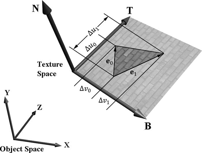
If you want to use a compressed texture format to store normal maps, then use the BC7 (DXGI_FORMAT_BC7_UNORM) format for the best quality, as it significantly reduces the errors caused by compressing normal maps. For BC6 and BC7 formats, the DirectX SDK has a sample called “BC6HBC7EncoderDecoder11.” This program can be used to convert your texture files to BC6 or BC7.

19.3 TEXTURE/TANGENT SPACE

Consider a 3D texture mapped triangle. For the sake of discussion, suppose that there is no distortion in the texture mapping; in other words, mapping the texture triangle onto the 3D triangle requires only a rigid body transformation (translation and rotation). Now, suppose that the texture is like a decal. So we pick the decal up, translate it, and rotate it onto the 3D triangle. Now Figure 19.4 shows how the texture space axes relate to the 3D triangle: they are tangent to the triangle and lie in the plane of the triangle. The texture coordinates of the triangle are, of course, relative to the texture space coordinate system. Incorporating the triangle face normal N, we obtain a 3D TBN-basis in the plane of the triangle that we call texture space or tangent space. Note that the tangent space generally varies from triangle-to-triangle (see Figure 19.5).

Figure 19.4. The relationship between the texture space of a triangle and the object space. The 3D tangent vector T aims in the u-axis direction of the texturing coordinate system, and the 3D tangent vector B aims in the v-axis direction of the texturing coordinate system.

Now, as Figure 19.3 shows, the normal vectors in a normal map are defined relative to the texture space. But our lights are defined in world space. In order to do lighting, the normal vectors and lights need to be in the same space. So our first step is to relate the tangent space coordinate system with the object space coordinate system the triangle vertices are relative to. Once we are in object space, we can use the world matrix to get from object space to world space (the details of this are covered in the next section). Let v₀, v₁, and v₂ define the three vertices of a 3D triangle with corresponding texture coordinates (u₀, v₀), (u₁, v₁), and (u₂, v₂) that define a triangle in the texture plane relative to the texture space axes (i.e., T and B). Let e₀ = v₁ − v₀ and e₁ = v₂ − v₀ be two edge vectors of the 3D triangle with corresponding texture triangle edge vectors (Δu₀, Δv₀) = (u₁ − u₀, v₁ − v₀) and (Δu₁, Δv₁) = (u₂ − u₀, v₂ − v₀) . From Figure 19.4, it is clear that

Representing the vectors with coordinates relative to object space, we get the matrix equation:

Note that we know the object space coordinates of the triangle vertices; hence we know the object space coordinates of the edge vectors, so the matrix

is known. Likewise, we know the texture coordinates, so the matrix

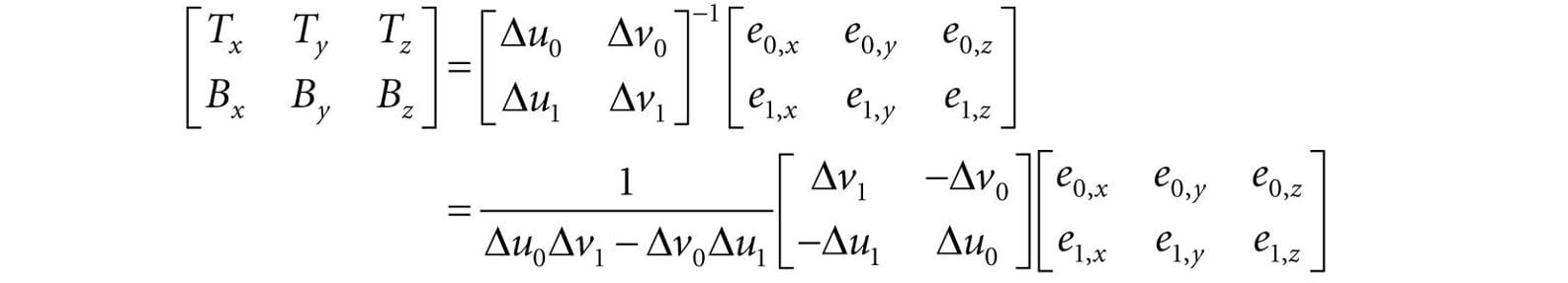
is known. Solving for the T and B object space coordinates we get:

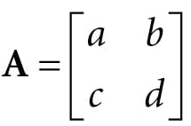
In the above, we used the fact that the inverse of a matrix

is given by:

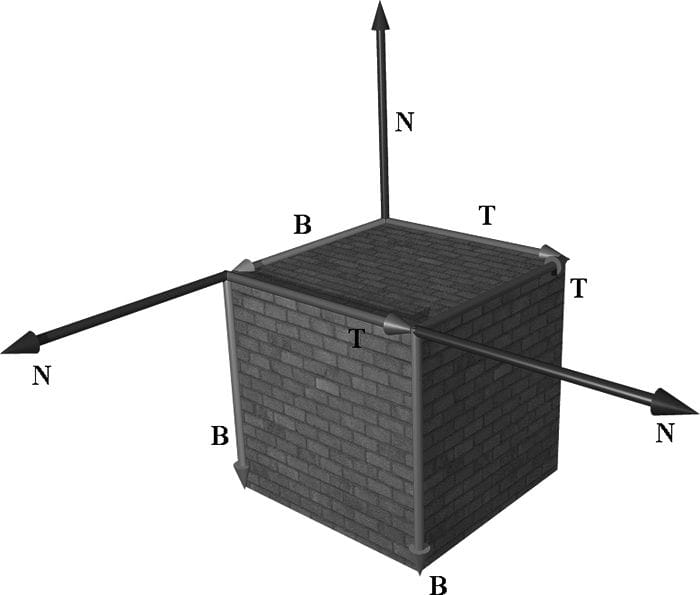
Note that the vectors T and B are generally not unit length in object space, and if there is texture distortion, they will not be orthonormal either.

The T, B, and N vectors are commonly referred to as the tangent, binormal (or bitangent), and normal vectors, respectively.

19.4 VERTEX TANGENT SPACE

In the previous section, we derived a tangent space per triangle. However, if we use this texture space for normal mapping, we will get a triangulated appearance since the tangent space is constant over the face of the triangle. Therefore, we specify tangent vectors per vertex, and we do the same averaging trick that we did with vertex normals to approximate a smooth surface:

1. The tangent vector T for an arbitrary vertex v in a mesh is found by averaging the tangent vectors of every triangle in the mesh that shares the vertex v.

2. The bitangent vector B for an arbitrary vertex v in a mesh is found by averaging the bitangent vectors of every triangle in the mesh that shares the vertex v.

Generally, after averaging, the TBN-bases will generally need to be orthonormalized, so that the vectors are mutually orthogonal and of unit length. This is usually done using the Gram-Schmidt procedure. Code is available on the web for building a per-vertex tangent space for an arbitrary triangle mesh: http://www.terathon.com/code/tangent.html.

In our system, we will not store the bitangent vector B directly in memory. Instead, we will compute B = N × T when we need B, where N is the usual averaged vertex normal. Hence, our vertex structure looks like this:

struct Vertex

{

XMFLOAT3 Pos;

XMFLOAT3 Normal;

XMFLOAT2 Tex;

XMFLOAT3 TangentU;

};

Recall that our procedurally generated meshes created by GeometryGenerator compute the tangent vector T corresponding to the u-axis of the texture space. The object space coordinates of the tangent vector T is easily specified at each vertex for box and grid meshes (see Figure 19.5). For cylinders and spheres, the tangent vector T at each vertex can be found by forming the vector-valued function of two variables P(u, v) of the cylinder/sphere and computing ∂p/∂u, where the parameter u is also used as the u-texture coordinate.

Figure 19.5. The texture space is different for each face of the box.

19.5 TRANSFORMING BETWEEN TANGENT SPACE AND OBJECT SPACE

At this point, we have an orthonormal TBN-basis at each vertex in a mesh. Moreover, we have the coordinates of the TBN vectors relative to the object space of the mesh. So now that we have the coordinate of the TBN-basis relative to the object space coordinate system, we can transform coordinates from tangent space to object space with the matrix:

Since this matrix is orthogonal, its inverse is its transpose. Thus, the change of coordinate matrix from object space to tangent space is:

In our shader program, we will actually want to transform the normal vector from tangent space to world space for lighting. One way would be to transform the normal from tangent space to object space first, and then use the world matrix to transform from object space to world space:

However, since matrix multiplication is associative, we can do it like this:

And note that

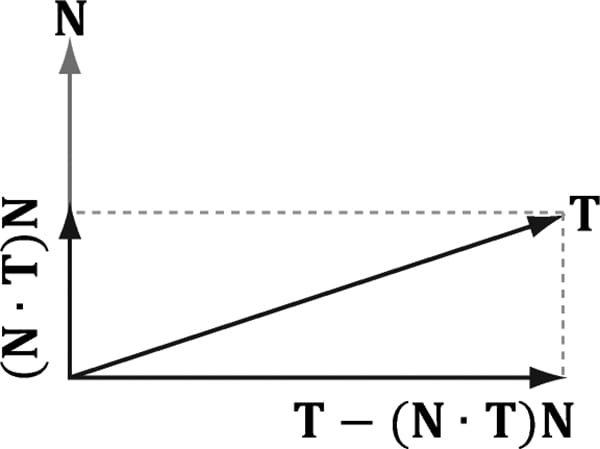
where

. So to go from tangent space directly to world space, we just have to describe the tangent basis in world coordinates, which can be done by transforming the TBN-basis from object space coordinates to world space coordinates.

We will only be interested in transforming vectors (not points). Thus, we only need a 3 × 3 matrix. Recall that the fourth row of an affine matrix is for translation, but we do not translate vectors.

19.6 NORMAL MAPPING SHADER CODE

We summarize the general process for normal mapping:

1. Create the desired normal maps from some art program or utility program and store them in an image file. Create 2D textures from these files when the program is initialized.

2. For each triangle, compute the tangent vector T. Obtain a per-vertex tangent vector for each vertex v in a mesh by averaging the tangent vectors of every triangle in the mesh that shares the vertex v. (In our demo, we use simply geometry and are able to specify the tangent vectors directly, but this averaging process would need to be done if using arbitrary triangle meshes made in a 3D modeling program.)

3. In the vertex shader, transform the vertex normal and tangent vector to world space and output the results to the pixel shader.

4. Using the interpolated tangent vector and normal vector, we build the TBN-basis at each pixel point on the surface of the triangle. We use this basis to transform the sampled normal vector from the normal map from tangent space to the world space. We then have a world space normal vector from the normal map to use for our usual lighting calculations.

To help us implement normal mapping, we have added the following function to Common.hlsl:

//--------------------------------------------------------------------

// Transforms a normal map sample to world space.

//--------------------------------------------------------------------

float3 NormalSampleToWorldSpace(float3 normalMapSample,

float3 unitNormalW,

float3 tangentW)

{

// Uncompress each component from [0,1] to [-1,1].

float3 normalT = 2.0f*normalMapSample - 1.0f;

// Build orthonormal basis.

float3 N = unitNormalW;

float3 T = normalize(tangentW - dot(tangentW, N)*N);

float3 B = cross(N, T);

float3x3 TBN = float3x3(T, B, N);

// Transform from tangent space to world space.

float3 bumpedNormalW = mul(normalT, TBN);

return bumpedNormalW;

}

This function is used like this in the pixel shader:

float3 normalMapSample = gNormalMap.Sample(samLinear, pin.Tex).rgb;

float3 bumpedNormalW = NormalSampleToWorldSpace(

normalMapSample,

pin.NormalW,

pin.TangentW);

Two lines that might not be clear are these:

float3 N = unitNormalW;

float3 T = normalize(tangentW - dot(tangentW, N)*N);

After the interpolation, the tangent vector and normal vector may not be orthonormal. This code makes sure T is orthonormal to N by subtracting off any component of T along the direction N (see Figure 19.6). Note that there is the assumption that unitNormalW is normalized.

Figure 19.6. Since ||N|| = 1, proj_N(T) = (T·N)N. The vector T-proj_N (T) is the portion of T orthogonal to N.

Once we have the normal from the normal map, which we call the “bumped normal,” we use it for all the subsequent calculation involving the normal vector (e.g., lighting, cube mapping). The entire normal mapping effect is shown below for completeness, with the parts relevant to normal mapping in bold.

//*********************************************************************

// Default.hlsl by Frank Luna (C) 2015 All Rights Reserved.

//*********************************************************************

// Defaults for number of lights.

#ifndef NUM_DIR_LIGHTS

#define NUM_DIR_LIGHTS 3

#endif

#ifndef NUM_POINT_LIGHTS

#define NUM_POINT_LIGHTS 0

#endif

#ifndef NUM_SPOT_LIGHTS

#define NUM_SPOT_LIGHTS 0

#endif

// Include common HLSL code.

#include “Common.hlsl”

struct VertexIn

{

float3 PosL : POSITION;

float3 NormalL : NORMAL;

float2 TexC : TEXCOORD;

float3 TangentU : TANGENT;

};

struct VertexOut

{

float4 PosH : SV_POSITION;

float3 PosW : POSITION;

float3 NormalW : NORMAL;

float3 TangentW : TANGENT;

float2 TexC : TEXCOORD;

};

VertexOut VS(VertexIn vin)

{

VertexOut vout = (VertexOut)0.0f;

// Fetch the material data.

MaterialData matData = gMaterialData[gMaterialIndex];

// Transform to world space.

float4 posW = mul(float4(vin.PosL, 1.0f), gWorld);

vout.PosW = posW.xyz;

// Assumes nonuniform scaling; otherwise, need to use

// inverse-transpose of world matrix.

vout.NormalW = mul(vin.NormalL, (float3x3)gWorld);

vout.TangentW = mul(vin.TangentU, (float3x3)gWorld);

// Transform to homogeneous clip space.

vout.PosH = mul(posW, gViewProj);

// Output vertex attributes for interpolation across triangle.

float4 texC = mul(float4(vin.TexC, 0.0f, 1.0f), gTexTransform);

vout.TexC = mul(texC, matData.MatTransform).xy;

return vout;

}

float4 PS(VertexOut pin) : SV_Target

{

// Fetch the material data.

MaterialData matData = gMaterialData[gMaterialIndex];

float4 diffuseAlbedo = matData.DiffuseAlbedo;

float3 fresnelR0 = matData.FresnelR0;

float roughness = matData.Roughness;

uint diffuseMapIndex = matData.DiffuseMapIndex;

uint normalMapIndex = matData.NormalMapIndex;

// Interpolating normal can unnormalize it, so renormalize it.

pin.NormalW = normalize(pin.NormalW);

float4 normalMapSample = gTextureMaps[normalMapIndex].Sample(

gsamAnisotropicWrap, pin.TexC);

float3 bumpedNormalW = NormalSampleToWorldSpace(

normalMapSample.rgb, pin.NormalW, pin.TangentW);

// Uncomment to turn off normal mapping.

//bumpedNormalW = pin.NormalW;

// Dynamically look up the texture in the array.

diffuseAlbedo *= gTextureMaps[diffuseMapIndex].Sample(

gsamAnisotropicWrap, pin.TexC);

// Vector from point being lit to eye.

float3 toEyeW = normalize(gEyePosW - pin.PosW);

// Light terms.

float4 ambient = gAmbientLight*diffuseAlbedo;

// Alpha channel stores shininess at per-pixel level.

const float shininess = (1.0f - roughness) * normalMapSample.a;

Material mat = { diffuseAlbedo, fresnelR0, shininess };

float3 shadowFactor = 1.0f;

float4 directLight = ComputeLighting(gLights, mat, pin.PosW,

bumpedNormalW, toEyeW, shadowFactor);

float4 litColor = ambient + directLight;

// Add in specular reflections.

float3 r = reflect(-toEyeW, bumpedNormalW);

float4 reflectionColor = gCubeMap.Sample(gsamLinearWrap, r);

float3 fresnelFactor = SchlickFresnel(fresnelR0, bumpedNormalW, r);

litColor.rgb += shininess * fresnelFactor * reflectionColor.rgb;

// Common convention to take alpha from diffuse albedo.

litColor.a = diffuseAlbedo.a;

return litColor;

}

Observe that the “bumped normal” vector is use in the light calculation, but also in the reflection calculation for modeling reflections from the environment map. In addition, in the alpha channel of the normal map we store a shininess mask, which controls the shininess at a per-pixel level (see Figure 19.7).

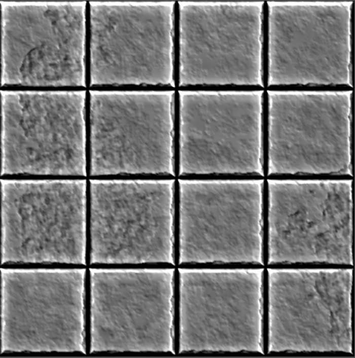
Figure 19.7. The alpha channel of the tile_nmap.dds image from the book’s DVD. The alpha channel denotes the shininess of the surface. White values indicate a shininess value of 1.0 and black values indicate a shininess value of 0.0. This gives us per-pixel control of the shininess material property.

19.7 SUMMARY

1. The strategy of normal mapping is to texture our polygons with normal maps. We then have per-pixel normals, which capture the fine details of a surface like bumps, scratches, and crevices. We then use these per-pixel normals from the normal map in our lighting calculations, instead of the interpolated vertex normal.

2. A normal map is a texture, but instead of storing RGB data at each texel, we store a compressed x-coordinate, y-coordinate, and z-coordinate in the red component, green component, and blue component, respectively. We use various tools to generate normal maps such as the ones located at http://developer.nvidia.com/nvidia-texture-tools-adobe-photoshop, http://www.crazybump.com/, and http://shadermap.com/home/.

3. The coordinates of the normals in a normal map are relative to the texture space coordinate system. Consequently, to do lighting calculations, we need to transform the normal from the texture space to the world space so that the lights and normals are in the same coordinate system. The TBN-bases built at each vertex facilitates the transformation from texture space to world space.

19.8 EXERCISES

1. Download the NVIDIA normal map plug-in (http://developer.nvidia.com/object/nv_texture_tools.html) and experiment with making different normal maps with it. Try your normal maps out in this chapter’s demo application.

2. Download the trial version of CrazyBump (http://www.crazybump.com/). Load a color image, and experiment making a normal and displacement map. Try your maps in this chapter’s demo application.

3. If you apply a rotation texture transformation, then you need to rotate the tangent space coordinate system accordingly. Explain why. In particular, this means you need to rotate T about N in world space, which will require expensive trigonometric calculations (more precisely, a rotation transform about an arbitrary axis N). Another solution is to transform T from world space to tangent space, where you can use the texture transformation matrix directly to rotate T, and then transform back to world space.

4. Instead of doing lighting in world space, we can transform the eye and light vector from world space into tangent space and do all the lighting calculations in that space. Modify the normal mapping shader to do the lighting calculations in tangent space.

5. The idea of displacement mapping is to utilize an additional map, called a heightmap, which describes the bumps and crevices of a surface. Often it is combined with hardware tessellation, where it indicates how newly added vertices should be offset in the normal vector direction to add geometric detail to the mesh. Displacement mapping can be used to implement ocean waves. The idea is to scroll two (or more) heightmaps over a flat vertex grid at different speeds and directions. For each vertex of the grid, we sample the heightmaps, and add the heights together; the summed height becomes the height (i.e., y-coordinate) of the vertex at this instance in time. By scrolling the heightmaps, waves continuously form and fade away giving the illusion of ocean waves (see Figure 19.8). For this exercise, implement the ocean wave effect just described using the two ocean wave heightmaps (and corresponding normal maps) available to download for this chapter (Figure 19.9). Here are a few hints to making the waves look good:

1. Tile the heightmaps differently so that one set can be used to model broad low frequency waves with high amplitude and the other can be used to model high frequency small choppy waves with low amplitude. So you will need two sets of texture coordinates for the heightmaps maps and two texture transformations for the heightmaps.

2. The normal map textures should be tiled more than the heightmap textures. The heightmaps give the shape of the waves, and the normal maps are used to light the waves per pixel. As with the heightmaps, the normal maps should translate over time and in different directions to give the illusion of new waves forming and fading. The two normals can then be combined using code similar to the following:

float3 normalMapSample0 = gNormalMap0.Sample(samLinear, pin.WaveNormalTex0).rgb;

float3 bumpedNormalW0 = NormalSampleToWorldSpace(

normalMapSample0, pin.NormalW, pin.TangentW);

float3 normalMapSample1 = gNormalMap1.Sample(samLinear, pin.WaveNormalTex1).rgb;

float3 bumpedNormalW1 = NormalSampleToWorldSpace(

normalMapSample1, pin.NormalW, pin.TangentW);

float3 bumpedNormalW = normalize(bumpedNormalW0 + bumpedNormalW1);

3. Modify the waves’ material to make it more ocean blue, and keep some reflection in from the environment map.

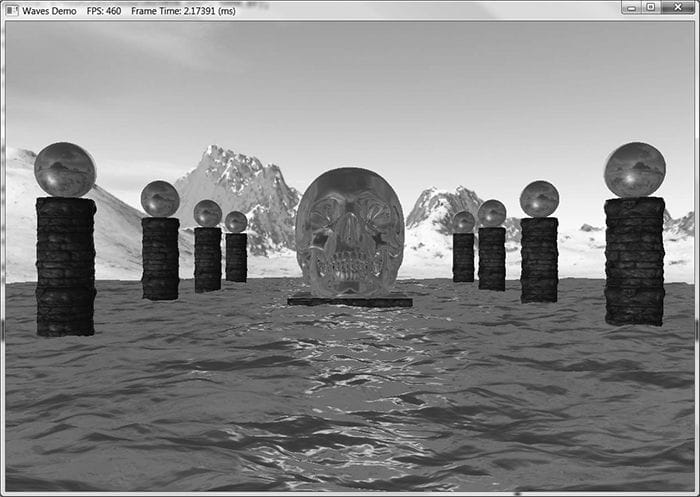
Figure 19.8. Ocean waves modeled with heightmaps, normal maps, and environment mapping.

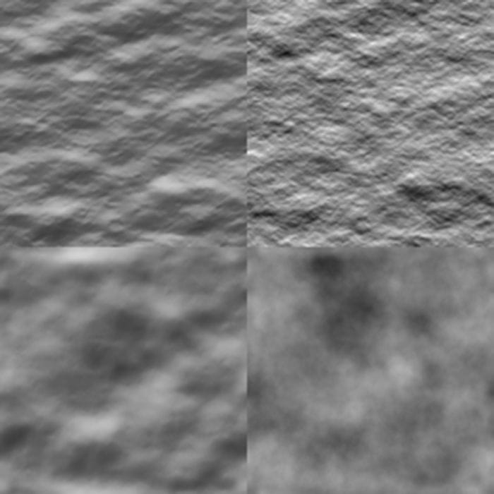
Figure 19.9. (Top Row) Ocean waves normal map and heightmap for high frequency choppy waves. (Bottom Row) Ocean waves normal map and heightmap for low frequency broad waves