Game Programming Algorithms and Techniques: A Platform-Agnostic Approach (2014)
Chapter 9. Artificial Intelligence
This chapter covers three major aspects of artificial intelligence in games: pathfinding, state-based behaviors, and strategy/planning. Pathfinding algorithms determine how non-player characters (NPCs) travel through the game world. State-based behaviors drive the decisions these characters make. Finally, strategy and planning are required whenever a large-scale AI plan is necessary, such as in a real-time strategy (RTS) game.
“Real” AI versus Game AI
In traditional computer science, much of the research on artificial intelligence (AI) has trended toward increasingly complex forms of AI, including genetic algorithms and neural networks. But such complex algorithms see limited use in computer and video games. There are two main reasons for this. The first issue is that complex algorithms require a great deal of computational time. Most games can only afford to spend a fraction of their total frame time on AI, which means efficiency is prioritized over complexity. The other major reason is that game AI typically has well-defined requirements or behavior, often at the behest of designers, whereas traditional AI is often focused on solving more nebulous and general problems.
In many games, AI behaviors are simply a combination of state machine rules with random variation thrown in for good measure. But there certainly are some major exceptions. The AI for a complex board game such as chess or Go requires a decision tree, which is a cornerstone of traditional game theory. But a board game with a relatively small number of possible moves at any one time is entirely different from the majority of video games. Although it’s acceptable for a chess AI to take several seconds to determine the optimal move, most games do not have this luxury. Impressively, there are some games that do implement more complex algorithms in real time, but these are the exception and not the rule. In general, AI in games is about perception of intelligence; as long as the player perceives that the AI enemies and companions are behaving intelligently, the AI system is considered a success.
It is also true that not every game needs AI. Some simple games, such as Solitaire and Tetris, certainly have no need for such algorithms. And even some more complex games may not require an AI, such as Rock Band. The same can be said for games that are 100% multiplayer and have noNPCs (non-player characters). But for any game where the design dictates that NPCs must react to the actions of the player, AI algorithms become a necessity.
Pathfinding
Pathfinding is the solution to a deceptively simple problem: Given points A and B, how does an AI intelligently traverse the game world between them?
The complexity of this problem stems from the fact that there can be a large set of paths between points A and B but only one path is objectively the best. For example, in Figure 9.1, both the red and blue paths are potential routes from point A to B. However, the blue path is objectively better than the red one, simply because it is shorter.
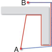
Figure 9.1 Two paths from A to B.
So it is not enough to simply find a single valid path between two points. The ideal pathfinding algorithm needs to search through all of the possibilities and find the absolute best path.
Representing the Search Space
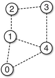
The simplest pathfinding algorithms are designed to work with the graph data structure. A graph contains a set of nodes, which can be connected to any number of adjacent nodes via edges. There are many different ways to represent a graph in memory, but the most basic is an adjacency list. In this representation, each node contains a list of pointers to any adjacent nodes. The entire set of nodes in the graph can then be stored in a standard container data structure. Figure 9.2 illustrates the visual and data representations of a simple graph.
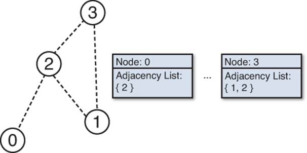
Figure 9.2 A sample graph.
This means that the first step to implement pathfinding in a game is to determine how the world will be represented as a graph. There are a several possibilities. A simple approach is to partition the world into a grid of squares (or hexes). The adjacent nodes in this case are simply the adjacent squares in the grid. This method is very popular for turn-based strategy games in the vein of Civilization or XCOM (see Figure 9.3).
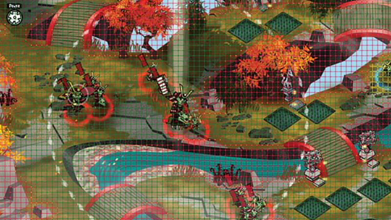
Figure 9.3 Skulls of the Shogun with its AI debug mode enabled to illustrate the square grid it uses for pathfinding.
However, for a game with real-time action, NPCs generally don’t move from square to square on a grid. Because of this, the majority of games utilize either path nodes or navigation meshes. With both of these representations, it is possible to manually construct the data in a level editor. But manually inputting this data can be tiresome and error prone, so most engines employ some automation in the process. The algorithms to automatically generate this data are beyond the scope of this book, though more information can be found in this chapter’s references.
Path nodes first became popular with the first-person shooter (FPS) games released by id Software in the early 1990s. With this representation, a level designer places path nodes at locations in the world that the AI can reach. These path nodes directly translate to the nodes in the graph. Automation can be employed for the edges. Rather than requiring the designer to stitch together the nodes by hand, an automated process can check whether or not a path between two relatively close nodes is obstructed. If there are no obstructions, an edge will be generated between these two nodes.
The primary drawback with path nodes is that the AI can only move to locations on the nodes or edges. This is because even if a triangle is formed by path nodes, there is no guarantee that the interior of the triangle is a valid location. There may be an obstruction in the way, so the pathfinding algorithm has to assume that any location that isn’t on a node or an edge is invalid.
In practice, this means that when path nodes are employed, there will be either a lot of unusable space in the world or a lot of path nodes. The first is undesirable because it results in less believable and organic behavior from the AI, and the second is simply inefficient. The more nodes and more edges there are, the longer it will take for a pathfinding algorithm to arrive at a solution. With path nodes, there is a very real tradeoff between performance and accuracy.
An alternative solution is to use a navigation mesh. In this approach, a single node in the graph is actually a convex polygon. Adjacent nodes are simply any adjacent convex polygons. This means that entire regions of a game world can be represented by a small number of convex polygons, resulting in a small number of nodes in the graph. Figure 9.4 compares how one particular room in a game would be represented by both path nodes and navigation meshes.
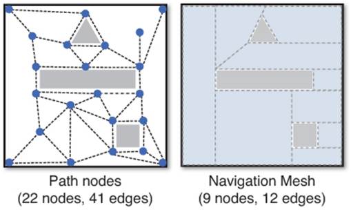
Figure 9.4 Two representations of the same room.
With a navigation mesh, any location contained inside one of the convex polygon nodes can be trusted. This means that the AI has a great deal of space to move around in, and as a result the pathfinding can return paths that look substantially more natural.
The navigation mesh has some additional advantages. Suppose there is a game where both cows and chickens walk around a farm. Given that chickens are much smaller than cows, there are going to be some areas accessible to the chickens, but not to the cows. If this particular game were using path nodes, it typically would need two separate graphs: one for each type of creature. This way, the cows would stick only to the path nodes they could conceivably use. In contrast, because each node in a navigation mesh is a convex polygon, it would not take very many calculations to determine whether or not a cow could fit in a certain area. Because of this, we can have only one navigation mesh and use our calculations to determine which nodes the cow can visit.
Add in the advantage that a navigation mesh can be entirely auto-generated, and it’s clear why fewer and fewer games today use path nodes. For instance, for many years the Unreal engine used path nodes for its search space representation. One such Unreal engine game that used path nodes was Gears of War. However, within the last couple of years the Unreal engine was retrofitted to use navigation meshes instead. Later games in the Gears of War series, such as Gears of War 3, used navigation meshes. This shift corresponds to the shift industry-wide toward the navigation mesh solution.
That being said, the representation of the search space does not actually affect the implementation of the pathfinding algorithm. As long as the search space can be represented by a graph, pathfinding can be attempted. For the subsequent examples in this section, we will utilize a grid of squares in the interest of simplicity. But the pathfinding algorithms will stay the same regardless of whether the representation is a grid of squares, path nodes, or a navigation mesh.
Admissible Heuristics
All pathfinding algorithms need a way to mathematically evaluate which node should be selected next. Most algorithms that might be used in a game utilize a heuristic, represented by h(x). This is the estimated cost from one particular node to the goal node. Ideally, the heuristic should be as close to the actual cost as possible. A heuristic is considered admissible if the estimate is guaranteed to always be less than or equal to the actual cost. If a heuristic overestimates the actual cost, there is decent probability that the pathfinding algorithm will not discover the best route.
For a grid of squares, there are two different ways to compute the heuristic, as shown in Figure 9.5. Manhattan distance is akin to travelling along city blocks in a sprawling metropolis. A particular building can be “five blocks away,” but that does not necessarily mean that there is only one route that is five blocks in length. Manhattan distance assumes that diagonal movement is disallowed, and because of this it should only be used as the heuristic if this is the case. If diagonal movement is allowed, Manhattan distance will often overestimate the actual cost.
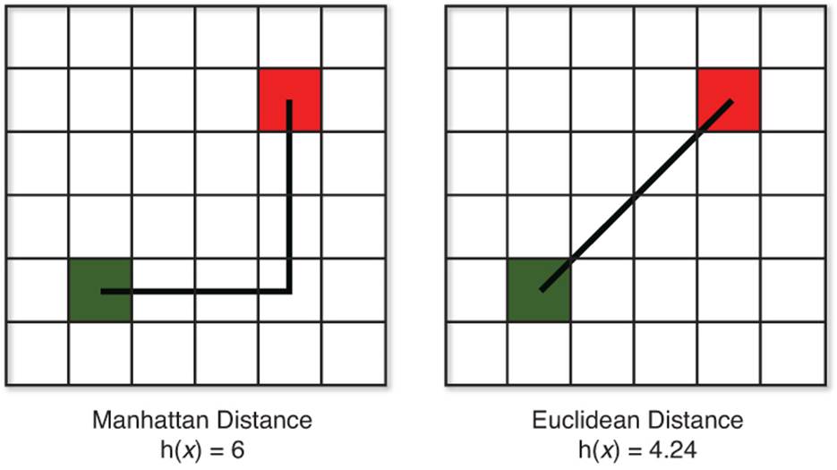
Figure 9.5 Manhattan and Euclidean heuristics.
In a 2D grid, the calculation for Manhattan distance is as follows:
h(x) = |start.x – end.x| + |start.y – end.y|
The second way to calculate a heuristic is Euclidean distance. This heuristic is calculated using the standard distance formula and estimates an “as the crow flies” route. Unlike Manhattan distance, Euclidean distance can also be employed in situations where another search space representation, such as path nodes or navigation meshes, is being utilized. In our same 2D grid, Euclidean distance is
![]()
Greedy Best-First Algorithm
Once there is a heuristic, a relatively basic pathfinding algorithm can be implemented: the greedy best-first search. An algorithm is considered greedy if it does not do any long-term planning and simply picks what’s the best answer “right now.” At each step of the greedy best-first search, the algorithm looks at all the adjacent nodes and selects the one with the lowest heuristic.
Although this may seem like a reasonable solution, the best-first algorithm can often result in sub-optimal paths. Take a look at the path presented in Figure 9.6. The green square is the starting node, the red square is the ending node, and grey squares are impassable. The arrows show the greedy best-first path.
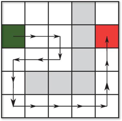
Figure 9.6 Greedy best-first path.
This path unnecessarily has the character travel to the right because, at the time, those were the best nodes to visit. An ideal route would have been to simply go straight down from the starting node, but this requires a level of planning the greedy-best first algorithm does not exhibit. Most games need better pathfinding than greedy best-first can provide, and because of this it does not see much use in actual games. However, the subsequent pathfinding algorithms covered in this chapter build on greedy best-first, so it is important you first understand how this algorithm is implemented before moving on.
First, let’s look at the data we need to store for each node. This data will be in addition to any adjacency data needed in order to construct the graph. For this algorithm, we just need a couple more pieces of data:
struct Node
Node parent
float h
end
The parent member variable is used to track which node was visited prior to the current one. Note that in a language such as C++, the parent would be a pointer, whereas in other languages (such as C#) classes may inherently be passed by reference. The parent member is valuable because it will be used to construct a linked list from the goal node all the way back to the starting node. When our algorithm is complete, the parent linked list will then be traversed in order to reconstruct the final path.
The float h stores the computed h(x) value for a particular node. This will be consulted when it is time to pick the node with the lowest h(x).
The next component of the algorithm is the two containers that temporarily store nodes: the open set and the closed set. The open set stores all the nodes that currently need to be considered. Because a common operation in our algorithm will be to find the lowest h(x) cost node, it is preferred to use some type of sorted container such as a binary heap or priority queue for the open set.
The closed set contains all of the nodes that have already been evaluated by the algorithm. Once a node is in the closed set, the algorithm stops considering it as a possibility. Because a common operation will be to check whether or not a node is already in the closed set, it may make sense to use a data structure in which a search has a time complexity better than O(n), such as a binary search tree.
Now we have the necessary components for a greedy best-first search. Suppose we have a start node and an end node, and we want to compute the path between the two. The majority of the work for the algorithm is processed in a loop. However, before we enter the loop, we need to initialize some data:
currentNode = startNode
add currentNode to closedSet
The current node simply tracks which node’s neighbors will be evaluated next. At the start of the algorithm, we have no nodes in our path other than the starting node. So it follows that we should first evaluate the neighbors of the starting node.
In the main loop, the first thing we want to do is look at all of the nodes adjacent to the current node and then add some of them to the open set:
do
foreach Node n adjacent to currentNode
if closedSet contains n
continue
else
n.parent = currentNode
if openSet does not contain n
compute n.h
add n to openSet
end
end
loop //end foreach
Note how any nodes already in the closed set are ignored. Nodes in the closed set have previously been fully evaluated, so they don’t need to be evaluated any further. For all other adjacent nodes, the algorithm sets their parent to the current node. Then, if the node is not already in the open set, we compute the h(x) value and add the node to the open set.
Once the adjacent nodes have been processed, we need to look at the open set. If there are no nodes left in the open set, this means we have run out of nodes to evaluate. This will only occur in the case of a pathfinding failure. There is no guarantee that there is always a solvable path, so the algorithm must take this into account:
if openSet is empty
break //break out of main loop
end
However, if we still have nodes left in the open set, we can continue. The next thing we need to do is find the lowest h(x) cost node in the open set and move it to the closed set. We also mark it as the current node for the next iteration of our loop.
currentNode = Node with lowest h in openSet
remove currentNode from openSet
add currentNode to closedSet
This is where having a sorted container for the open set becomes handy. Rather than having to do an O(n) search, a binary heap will grab the lowest h(x) node in O(1) time.
Finally, we have the exit case of the loop. Once we find a valid path, the current node will be the same as the end node, at which point we can finish the loop.
until currentNode == endNode //end main do...until loop
If we exit the do...until loop in the success case, we will have a linked list of parents that take us from the end node all the way back to the start node. Because we want a path from the start node to the end node, we must reverse it. There are several ways to reverse the list, but one of the easiest is to use a stack.
Figure 9.7 shows the first two iterations of the greedy best-first algorithm applied to the sample data set. In Figure 9.7(a), the start node has been added to the closed set, and its adjacent nodes (in blue) are added to the open set. Each adjacent node has its h(x) cost to the end node calculated with the Manhattan distance heuristic. The arrows point from the children back to their parent. The next part of the algorithm is to select the node with the lowest h(x) cost, which in this case is the node with h = 3. It gets marked as the current node and is moved to the closed set. Figure 9.7(b)then shows the next iteration, with the nodes adjacent to the current node (in yellow) added to the open set.
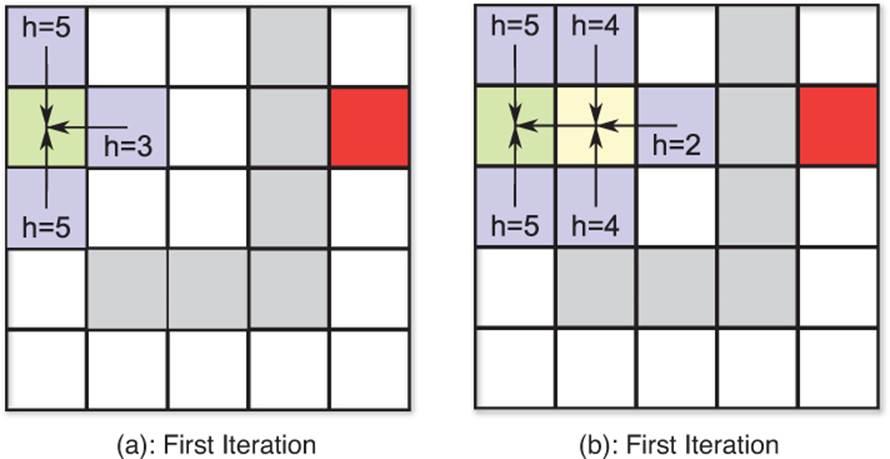
Figure 9.7 Greedy best-first snapshots.
Once the goal node (in red) is added to the closed set, we would then have a linked list from the end node all the way back to the starting node. This list can then be reversed in order to get the path illustrated earlier in Figure 9.6.
The full listing for the greedy best-first algorithm follows in Listing 9.1. Note that this implementation makes the assumption that the h(x) value cannot change during the course of execution.
Listing 9.1 Greedy Best-First Algorithm
curentNode = startNode
add currentNode to closedSet
do
// Add adjacent nodes to open set
foreach Node n adjacent to currentNode
if closedSet contains n
continue
else
n.parent = currentNode
if openSet does not contain n
compute n.h
add n to openSet
end
end
loop
// All possibilities were exhausted
if openSet is empty
break
end
// Select new current node
currentNode = Node with lowest h in openSet
remove currentNode from openSet
add currentNode to closedSet
until currentNode == endNode
// If the path was solved, reconstruct it using a stack reversal
if currentNode == endNode
Stack path
Node n = endNode
while n is not null
push n onto path
n = n.parent
loop
else
// Path unsolvable
end
If we want to avoid the stack reversal to reconstruct the path, another option is to instead calculate the path from the goal node to the start node. This way, the linked list that we end up with will be in the correct order from the start node to the goal node, which can save some computation time. This optimization trick is used in the tower defense game in Chapter 14, “Sample Game: Tower Defense for PC/Mac” (though it does not implement greedy-best first as its pathfinding algorithm).
A* Pathfinding
Now that we’ve covered the greedy best-first algorithm, we can add a bit of a wrinkle to greatly improve the quality of the path. Instead of solely relying on the h(x) admissible heuristic, the A* algorithm (pronounced A-star) adds a path-cost component. The path-cost is the actual cost from the start node to the current node, and is denoted by g(x). The equation for the total cost to visit a node in A* then becomes:
f(x) = g(x) + h(x)
In order for us to employ the A* algorithm, the Node struct needs to additionally store the f(x) and g(x) values, as shown:
struct Node
Node parent
float f
float g
float h
end
When a node is added to the open set, we must now calculate all three components instead of only the heuristic. Furthermore, the open set will instead be sorted by the full f(x) value, as in A* we will select the lowest f(x) cost node every iteration.
There is only one other major change to the code for the A* algorithm, and that is the concept of node adoption. In the best-first algorithm, adjacent nodes always have their parent set to the current node. However in A*, adjacent nodes that are already in the open set need to have their value evaluated to determine whether the current node is a superior parent.
The reason for this is that the g(x) cost of a particular node is dependent on the g(x) cost of its parent. This means that if a more optimal parent is available, the g(x) cost of a particular node can be reduced. So we don’t want to automatically replace a node’s parent in A*. It should only be replaced when the current node is a better parent.
In Figure 9.8(a), we see the current node (in teal) checking its adjacent nodes. The node to its left has g = 2. If that node instead had teal as its parent, it would have g = 4, which is worse. So in this case, the node in teal has its adoption request denied. Figure 9.8(b) shows the final path as computer by A*, which is clearly superior to the greedy best-first solution.
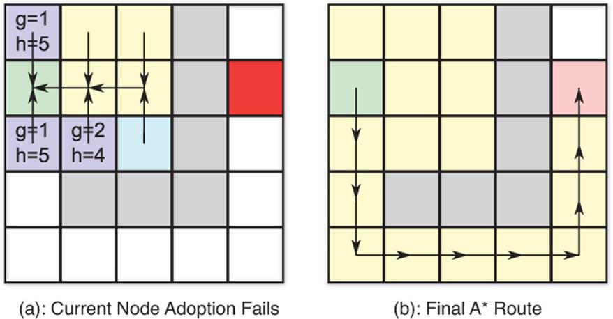
Figure 9.8 A* path.
Apart from the node adoption, the code for the A* algorithm ends up being very similar to best-first, as shown in Listing 9.2.
Listing 9.2 A* Algorithm
currentNode = startNode
add currentNode to closedSet
do
foreach Node n adjacent to currentNode
if closedSet contains n
continue
else if openSet contains n // Check for adoption
compute new_g // g(x) value for n with currentNode as parent
if new_g < n.g
n.parent = currentNode
n.g = new_g
n.f = n.g + n.h // n.h for this node will not change
end
else
n.parent = currentNode
compute n.h
compute n.g
n.f = n.g + n.h
add n to openSet
end
loop
if openSet is empty
break
end
currentNode = Node with lowest f in openSet
remove currentNode from openSet
add currentNode to closedSet
until currentNode == endNode
// Path reconstruction from Listing 9.1.
...
The tower defense game covered in Chapter 14 provides a full implementation of the A* algorithm over a hex-based grid.
Dijkstra’s Algorithm
One final pathfinding algorithm can be implemented with only a minor modification to A*. In Dijkstra’s algorithm, there is no heuristic estimate—or in other words:
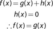
This means that Dijkstra’s algorithm can be implemented with the same code as A* if we use zero as the heuristic. If we apply Dijkstra’s algorithm to our sample data set, we get a path that is identical to the one generated by A*. Provided that the heuristic used for A* was admissible, Dijkstra’s algorithm will always return the same path as A*. However, Dijkstra’s algorithm typically ends up visiting more nodes, which means it’s less efficient than A*.
The only scenario where Dijkstra’s might be used instead of A* is when there are multiple valid goal nodes, but you have no idea which one is the closest. But that scenario is rare enough that most games do not use Dijkstra’s; the algorithm is mainly discussed for historical reasons, as Dijkstra’s algorithm actually predates A* by nearly ten years. A* was an innovation that combined both the greedy best-first search and Dijkstra’s algorithm. So even though this book covers Dijkstra’s through the lens of A*, that is not how it was originally developed.
State-Based Behaviors
The most basic AI behavior has no concept of different states. Take for instance an AI for Pong: It only needs to track the position of the ball. This behavior never changes throughout the course of the game, so such an AI would be considered stateless. But add a bit more complexity to the game, and the AI needs to behave differently at different times. Most modern games have NPCs that can be in one of many states, depending on the situation. This section discusses how to design an AI with states in mind, and covers how these state machines might be implemented.
State Machines for AI
A finite state machine is a perfect model to represent the state-based behavior of an AI. It has a set number of possible states, conditions that cause transitions to other states, and actions that can be executed upon entering/exiting the state.
When you’re implementing a state machine for an AI, it makes sense to first plan out what exactly the different behaviors should be and how they should be interconnected. Suppose we are implementing a basic AI for a guard in a stealth-based game. By default, we want the guard to patrol along a set path. If the guard detects the player while on patrol, it should start attacking the player. And, finally, if in either state the guard is killed, it should die. The AI as described should therefore have three different states: Patrol, Attack, and Death.
Next, we need to determine which transitions are necessary for our state machine. The transition to the Death state should be apparent: When the guard’s killed, it’ll enter the Death state. As for the Attack state, the only time it should be entered is if the player is spotted while the guard is patrolling. Combine these criteria together, and we can draw a simple flow chart for our state machine, as in Figure 9.9.
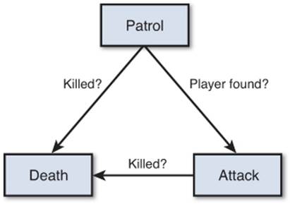
Figure 9.9 Basic stealth AI state machine.
Although this AI would be functional, it is lacking compared to the AI in most stealth games. Suppose the guard is patrolling and hears a suspicious sound. In our current state machine, the AI would go about its business with no reaction. Ideally, we would want an “Investigate” state, where the AI starts searching for the player in that vicinity. Furthermore, if the guard detects the player, it currently always attacks. Perhaps we instead want an “Alert” state that, upon being entered, randomly decides whether to start attacking or to trigger an alarm.
If we add in these elements, our state machine starts to become more complex, as in Figure 9.10.
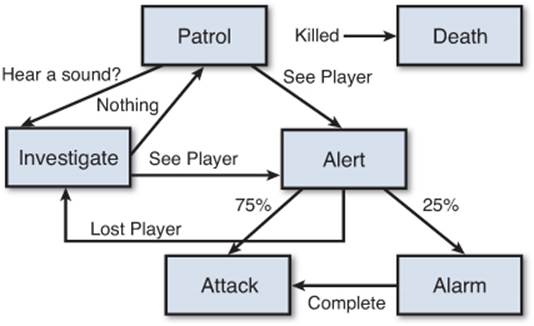
Figure 9.10 More complex stealth AI state machine.
Notice how the Death state has been detached from the others. This was done simply to remove some arrows from the flow chart, because any state can transition into the Death state when the AI is killed. Now, we could add even more complexities to our AI’s behavior if we so desired. But the principles of designing an AI’s behavior are the same irrespective of the number of states.
Ghost AI in Pac-Man
At first glance, it may seem like the AI for the arcade classic Pac-Man is very basic. The ghosts appear to either chase after the player or run from the player, so one might think that it’s just a binary state machine. However, it turns out that the ghost AI is relatively complex.
Toru Iwatani, designer of Pac-Man, spoke with Susan Lammers on this very topic in her 1986 book Programmers at Work. He “wanted each ghostly enemy to have a specific character and its own particular movements, so they weren’t all just chasing after Pac-Man...which would have been tiresome and flat.”
Each of the four ghosts have four different behaviors to define different target points in relation to Pac-Man or the maze. The ghosts also alternate between phases of attacking and dispersing, with the attack phases increasing proportionally as the player progresses to further and further levels.
An excellent write up on the implementation of the Pac-Man ghost AI is available on the Game Internals blog at http://tinyurl.com/238l7km.
Basic State Machine Implementation
A state machine can be implemented in several ways. A minimum requirement is that when the AI updates itself, the correct update action must be performed based on the current state of the AI. Ideally, we would also like our state machine implementation to support enter and exit actions.
If the AI only has two states, we could simply use a Boolean check in the AI’s Update function. But this solution is not very robust. A slightly more flexible implementation, often used in simple games, is to have an enumeration (enum) that represents all of the possible states. For instance, an enum for the states in Figure 9.9 would be the following:
enum AIState
Patrol,
Death,
Attack
end
We could then have an AIController class with a member variable of type AIState. In our AIController’s Update function, we could simply perform the current action based on the current state:
function AIController.Update(float deltaTime)
if state == Patrol
// Perform Patrol actions
else if state == Death
// Perform Death actions
else if state == Attack
// Perform Attack actions
end
end
State changes and enter/exit behaviors could then be implemented in a second function:
function AIController.SetState(AIState newState)
// Exit actions
if state == Patrol
// Exit Patrol state
else if state == Death
// Exit Death state
else if state == Attack
// Exit Attack state
end
state = newState
// Enter actions
if state == Patrol
// Enter Patrol state
else if state == Death
// Enter Death state
else if state == Attack
// Enter Attack state
end
end
There are a number of issues with this implementation. First and foremost, as the complexity of our state machine increases, the readability of the Update and SetState functions decrease. If we had 20 states instead of the three in this example, the functions would end up looking like spaghetti code.
A second major problem is the lack of flexibility. Suppose we have two different AIs that have largely different state machines. This means that we would need to have a different enum and controller class for each of the different AIs. Now, suppose it turns out that both of these AIs do share a couple of states in common, most notably the Patrol state. With the basic state machine implementation, there isn’t a great way to share the Patrol state code between both AI controllers.
One could simply copy the Patrol code into both classes, but having nearly identical code in two separate locations is never a good practice. Another option might be to make a base class that each AI inherits from and then “bubble up” the majority of the Patrol behavior to this base class. But this, too, has drawbacks: It means that any subsequent AI that needs a Patrol behavior also must inherit from this shared class.
So even though this basic implementation is functional, it is not recommended for more than the simplest of AI state machines.
State Design Pattern
A design pattern is a generalized solution to a commonly occurring problem. The seminal book on design patterns is the so-called “Gang of Four” Design Patterns book, which is referenced at the end of this chapter. One of the design patterns is the State pattern, which allows “an object to alter its behavior when its internal state changes.”
This can be implemented using class composition. So the AIController “has-a” AIState as a member variable. Each specific state then subclasses AIState. Figure 9.11 shows a rough class diagram.
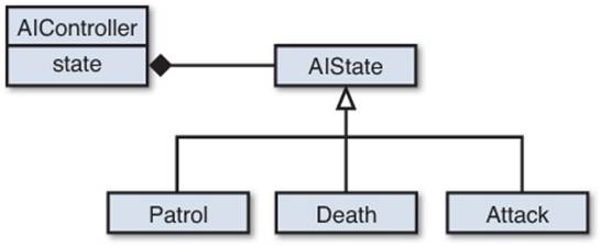
Figure 9.11 State design pattern.
The AIState base class could then be defined as follows:
class AIState
AIController parent
function Update(float deltaTime)
function Enter()
function Exit()
end
The parent reference allows a particular instance of an AIState to keep track of which AIController owns it. This is required because if we want to switch into a new state, there has to be some way to notify the AIController of this. Each AIState also has its own Update,Enter, and Exit functions, which can implement state-specific actions.
The AIController class could then have a reference to the current AIState and the required Update and SetState functions:
class AIController
AIState state
function Update(float deltaTime)
function SetState(AIState newState)
end
This way, the AIController’s Update function can simply call the current state’s Update:
function AIController.Update(float deltaTime)
state.Update(deltaTime)
end
With the design pattern implementation, the SetState function is also much cleaner:
function AIController.SetState(AIState newState)
state.Exit()
state = newState
state.Enter()
end
With the state design pattern, all state-specific behavior is moved into the subclasses of AIState. This makes the AIController code much cleaner than in the previous implementation. The State design pattern also makes the system far more modular. For instance, if we wanted to use the Patrol code in multiple state machines, it could be dropped in relatively easily. And even if we needed slightly different Patrol behavior, the Patrol state could be subclassed.
Strategy and Planning
Certain types of games require AI that is more complex than state-based enemies. In genres such as real-time strategy (RTS), the AI is expected to behave in a manner similar to a human player. The AI needs to have an overarching vision of what it wants to do, and then be able to act on that vision. This is where strategy and planning come into play. In this section, we will take a high-level look at strategy and planning through the lens of the RTS genre, though the techniques described could apply to other genres as well.
Strategy
Strategy is an AI’s vision of how it should compete in the game. For instance, should it be more aggressive or more defensive? In an RTS game, there are often two components of strategy: micro and macro strategy. Micro strategy consists of per-unit actions. This can typically be implemented with behavioral state machines, so it is nothing that requires further investigation. Macro strategy, however, is a far more complex problem. It is the AI’s overarching strategy, and it determines how it wants to approach the game. When programming AIs for games such asStarCraft, developers often model the strategy after top professional players. An example of a macro strategy in an RTS game might be to “rush” (try to attack the other player as quickly as possible).
Strategies can sometimes seem like nebulous mission statements, and vague strategies are difficult to program. To make things more tangible, strategies are often thought in terms of specific goals. For example, if the strategy is to “tech” (increase the army’s technology), one specific goal might be to “expand” (create a secondary base).
Note
Full-game RTS AI strategy can be extremely impressive when implemented well. The annual Artificial Intelligence and Interactive Digital Entertainment (AIIDE) conference has a StarCraft AI competition. Teams from different universities create full-game AI bots that fight it out over hundreds of games. The results are quite interesting, with the AI displaying proficiency that approaches that of an experienced player. More information as well as videos are available here at www.starcraftaicompetition.com.
A single strategy typically has more than one goal. This means that we need a prioritization system to allow the AI to pick which goal is most important. All other goals would be left on the back burner while the AI attempts to achieve its highest priority one. One way to implement a goal system would be to have a base AIGoal class as such this:
class AIGoal
function CalculatePriority()
function ConstructPlan()
end
Each specific goal would then be implemented as a subclass of AIGoal. So when a strategy is selected, all of that strategy’s goals would be added to a container that is sorted by priority. Note that a truly advanced strategy system should support the idea of multiple goals being active at once. If two goals are not mutually exclusive, there is no reason why the AI should not attempt to achieve both goals at the same time.
The heuristic for calculating the priority in CalculatePriority may be fairly complex, and will be wildly different depending on the game rules. For instance, a goal of “build air units” may have its priority reduced if the AI discovers that the enemy is building units that can destroy air units. By the same token, its priority may increase if the AI discovers the enemy has no anti-air capabilities.
The ConstructPlan function in AIGoal is responsible for constructing the plan: the series of steps that need to be followed in order to achieve the desired goal.
Planning
Each goal will need to have a corresponding plan. For instance, if the goal is to expand, then the plan may involve the following steps:
1. Scout for a suitable location for an expansion.
2. Build enough units to be able to defend the expansion.
3. Send a worker plus the defender units to the expansion spot.
4. Start building the expansion.
The plan for a specific goal could be implemented by a state machine. Each step in the plan could be a state in the state machine, and the state machine can keep updating a particular step until the condition is met to move on to the next state. However, in practice a plan can rarely be so linear. Based on the success or failure of different parts of the plan, the AI may have to modify the ordering of its steps.
One important consideration is that the plan needs to periodically assess the goal’s feasibility. If during our expansion plan it is discovered that there are no suitable expansion locations, then the goal cannot be achieved. Once a goal is flagged as unachievable, the overarching strategy also needs to be reevaluated. Ultimately, there is the necessity of having a “commander” who will decide when the strategy should be changed.
The realm of strategy and planning can get incredibly complex, especially if it’s for a fully featured RTS such as StarCraft. For further information on this topic, check the references at the end of this chapter.
Summary
The goal of a game AI programmer is to create a system that appears to be intelligent. This may not be what a researcher considers “true” AI, but games typically do not need such complex AIs. As we discussed, one big problem area in game AI is finding the best path from point A to point B. The most common pathfinding algorithm used in games is A*, and it can be applied on any search space that can be represented by a graph (which includes a grid, path nodes, or navigation meshes). Most games also have some sort of AI behavior that is controlled by a state machine, and the best way to implement a state machine is with the State design pattern. Finally, strategy and planning may be utilized by genres such as RTS in order to create more organic and believable opponents.
Review Questions
1. Given the following graph, what are the adjacency lists for each node?
2. Why are navigation meshes generally preferred over path nodes?
3. When is a heuristic considered admissible?
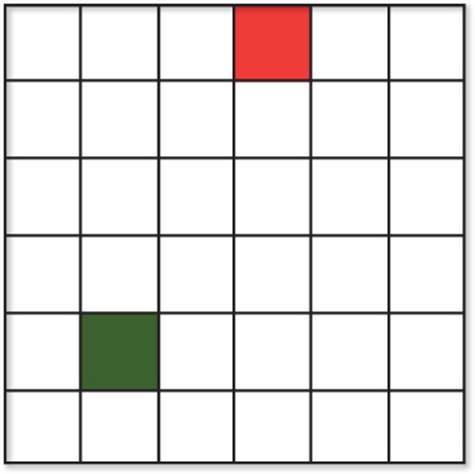
4. Calculate the Manhattan and Euclidean distances between the red and green nodes in the following diagram:
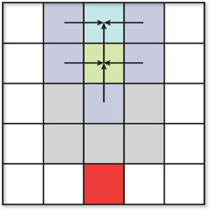
5. The A* algorithm is being applied to the following data. Nodes adjacent to the current node have been added, so the algorithm needs to select a new current node. Calculate the f(x) cost of each node in the open set (in blue) using a Manhattan heuristic, and assume diagonal travel is not allowed. Which node is selected as the new current node?
6. If the A* algorithm has its heuristic changed such that h(x) = 0, which algorithm does this mimic?
7. Compare A* to Dijkstra’s algorithm. Is one preferred over the other, and why?
8. You are designing an AI for an enemy wolf. Construct a simple behavioral state machine for this enemy with at least five states.
9. What are the advantages of the state design pattern?
10. What is a strategy, and how can it be broken down into smaller components?
Additional References
General AI
Game/AI (http://ai-blog.net/). This blog has articles from several programmers with industry experience who talk about many topics related to AI programming.
Millington, Ian and John Funge. Artificial Intelligence for Games (2nd Edition). Burlington: Morgan Kaufmann, 2009. This book is an algorithmic approach to many common game AI problems.
Game Programming Gems (Series). Each volume of this series has a few articles on AI programming. The older volumes are out of print, but the newer ones are still available.
AI Programming Wisdom (Series). Much like the Game Programming Gems series, except 100% focused on AI for games. Some of the volumes are out of print.
Pathfinding
Recast and Detour (http://code.google.com/p/recastnavigation/). An excellent open source pathfinding library written by Mikko Mononen, who has worked on several games including Crysis. Recast automatically generates navigation meshes, and Detour implements pathfinding within the navigation mesh.
States
Gamma, Eric et. al. Design Patterns: Elements of Reusable Object-Oriented Software. Boston: Addison-Wesley, 1995. Describes the state design pattern as well as many other design patterns. Useful for any programmer.
Buckland, Mat. Programming Game AI By Example. Plano: Wordware Publishing, 2005. This is a general game AI book, but it also has great examples of state-based behavior implementations.
All materials on the site are licensed Creative Commons Attribution-Sharealike 3.0 Unported CC BY-SA 3.0 & GNU Free Documentation License (GFDL)
If you are the copyright holder of any material contained on our site and intend to remove it, please contact our site administrator for approval.
© 2016-2026 All site design rights belong to S.Y.A.