Game Programming Algorithms and Techniques: A Platform-Agnostic Approach (2014)
Chapter 4. 3D Graphics
Although the first 3D games were released in the arcade era, it wasn’t really until the mid-to-late 1990s that 3D took off. Today, nearly all AAA titles on consoles and PCs are 3D games. And as the power of smartphones increases, more and more mobile games are as well.
The primary technical challenge of a 3D game is displaying the game world’s 3D environment on a flat 2D screen. This chapter discusses the building blocks necessary to accomplish this.
Basics
The first 3D games needed to implement all their rendering in software. This meant that even something as basic as drawing a line had to be implemented by a graphics programmer. The set of algorithms necessary to draw 3D objects into a 2D color buffer are collectively known as software rasterization, and most courses in computer graphics spend some amount of time discussing this aspect of 3D graphics. But modern computers have dedicated graphics hardware, known as the graphics processing unit (GPU), that knows how to draw basic building blocks such as points, lines, and triangles.
Because of this, modern games do not need to implement software rasterization algorithms. The focus is instead on giving the graphics card the data it needs to render the 3D scene in the desired manner, using libraries such as OpenGL and DirectX. And if further customization is necessary, custom micro-programs, known as shaders, can be applied to this data as well. But once this data is put together, the graphics card will take it and draw it on the screen for you. The days of coding out Bresenham’s line-drawing algorithm are thankfully gone.
One thing to note is that in 3D graphics, it’s often necessary to use approximations. This is because there simply isn’t enough time to compute photorealistic light. Games are not like CG films, where hours can be spent to compute one single frame. A game needs to be drawn 30 or 60 times per second, so accuracy must be compromised in favor of performance. A graphical error that is the result of an approximation is known as a graphical artifact, and no game can avoid artifacts entirely.
Polygons
3D objects can be represented in a computer program in several ways, but the vast majority of games choose to represent their 3D objects with polygons—specifically, triangles.
Why triangles? First of all, they are the simplest polygon possible because they can be represented by only three vertices, or the points on the corners of the polygon. Second, triangles are guaranteed to lie on a single plane, whereas a polygon with four or more vertices may lie on multiple planes. Finally, arbitrary 3D objects easily tessellate into triangles without leaving holes or other deformations.
A single model, or mesh, is made up of a large number of triangles. The number of triangles a particular mesh has depends on the platform constraints as well as the particular use of the model. For an Xbox 360 game, a character model may have 15,000 polygons, whereas a barrel might be represented by a couple hundred. Figure 4.1 shows a mesh represented with triangles.
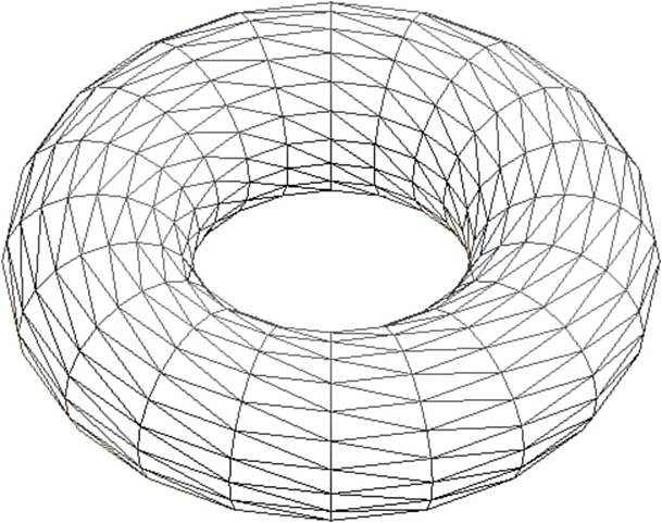
Figure 4.1 A sample mesh made with triangles.
All graphics libraries have some way to specify the lists of triangles we want the graphics card to render. We then must also provide further information regarding how we want these list of triangles to be drawn, which is what the rest of this chapter covers.
Coordinate Spaces
A coordinate space provides a frame of reference to a particular scene. For example, in the Cartesian coordinate space, the origin is known to be in the center of the world, and positions are relative to that center. In a similar manner, there can be other coordinate spaces relative to different origins. In the 3D rendering pipeline, we must travel through four primary coordinate spaces in order to display a 3D model on a 2D monitor:
![]() Model
Model
![]() World
World
![]() View/camera
View/camera
![]() Projection
Projection
Model Space
When a model is created, whether procedurally or in a program such as Maya, all the vertices of the model are expressed relative to the origin of that model. Model space is this coordinate space that’s relative to the model itself. In model space, the origin quite often is in the center of the model—or in the case of a humanoid, between its feet. That’s because it makes it easier to manipulate the object if its origin is centered.
Now suppose there are 100 different objects in a particular game’s level. If the game loaded up the models and just drew them at their model space coordinates, what would happen? Well, because every model was created at the origin in model space, every single object, including the player, would be at the origin too! That’s not going to be a particularly interesting level. In order for this level to load properly, we need another coordinate system.
World Space
This new coordinate system is known as world space. In world space, there is an origin for the world as a whole, and every object has a position and orientation relative to that world origin.
When a model is loaded into memory, all its vertices are expressed in terms of model space. We don’t want to manually change that vertex data in memory, because it would result in poor performance and would prevent positioning multiple instances of the model at several locations in the world.
What we want instead is a way to tell the graphics card where we want the particular model to be drawn. And it’s not just location: some models may need to be rotated differently, some may need to be scaled, and so on (as demonstrated in Figure 4.2). So the desired solution would be to pass the model data (in model space) to the graphics card as well as the little bit of additional data needed place the model in the world.
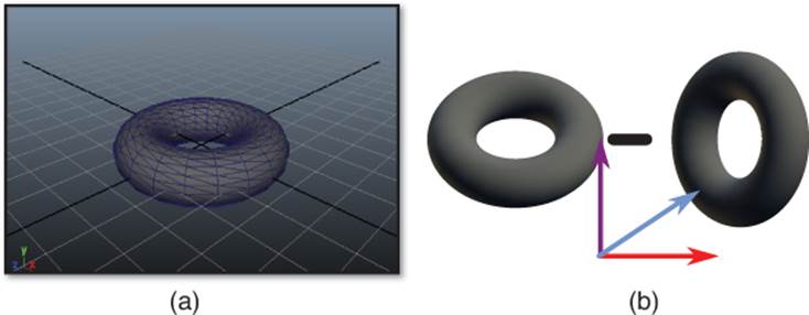
Figure 4.2 Object in model space (a), and several instances of the object positioned/oriented relative to world space (b).
It turns out that for that extra bit of data, we are going to use our trusty matrices. But first, before we can use matrices we need a slightly different way to represent the positions of the triangles, called homogenous coordinates.
Homogenous Coordinates
As mentioned earlier, sometimes 3D games will actually use 4D vectors. When 4D coordinates are used for a 3D space, they are known as homogenous coordinates, and the fourth component is known as the w-component.
In most instances, the w-component will be either 0 or 1. If w = 0, this means that the homogenous coordinate represents a 3D vector. On the other hand, if w = 1, this means that the coordinate represents a 3D point. However, what’s confusing is that in code you will typically see a class such as Vector4 used both for vectors or points. Due to this, it is very important that the vectors are named in a sensible manner, such as this:
Vector4 playerPosition // This is a point
Vector4 playerFacing // This is a vector
Transforming 4D Vectors by Matrices
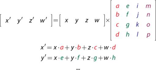
The matrices we use to transform objects will often be 4×4 matrices. But in order to multiply a vector by a 4×4 matrix, the vector has to be 4D, as well. This is where homogenous coordinates come into play.
Multiplying a 4D vector by a 4×4 matrix is very similar to multiplying a 3D vector by a 3×3 matrix:
Once you understand how to transform a 4D homogenous coordinate by a matrix, you can then construct matrices in order to perform the specific transformations you want in world space.
Transform Matrices
A transform matrix is a matrix that is able to modify a vector or point in a specific way. Transform matrices are what allow us to have model space coordinates transformed into world space coordinates.
As a reminder, all of these transform matrices are presented in row-major representations. If you are using a library that expects a column-major representation (such as OpenGL), you will need to transpose these matrices. Although the matrices that follow are presented in their 4×4 forms, the scale and rotation matrices can have their fourth row/column removed if a 3×3 matrix is desired instead.
Scale
Suppose we have a player character model that was created to be a certain size. In game, there is a power-up that can double the size of the character. This means we need to be able to increase the size of the model in world space. This could be accomplished by multiplying every vertex in the model by an appropriate scale matrix, which can scale a vector or position along any of the three coordinate axes. It looks a lot like the identity matrix, except the diagonal comprises the scale factors.
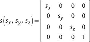
If sx = sy = sz, this is a uniform scale, which means the vector is transformed equally along all axes. So if all the scale values are 2, the model will double in size.
To invert a scale matrix, simply take the reciprocal of each scale factor.
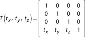
Translation
A translation matrix moves a point by a set amount. It does not work on vectors, because the value of a vector does not depend on where we draw the vector. The translation matrix fills in the final row of the identity matrix with the x, y, and z translation values.
For example, suppose the center of a model is to be placed at the position ![]() 5, 10, –15
5, 10, –15![]() in the world. The matrix for this translation would be as follows:
in the world. The matrix for this translation would be as follows:
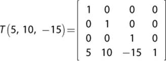
This matrix will have no effect on a vector because the homogenous representation of a vector has a w-component of 0. This means that the fourth row of the translation matrix would be cancelled out when the vector and matrix are multiplied. But for points, the w-component is typically 1, which means the translation components will be added in.
To invert a translation matrix, negate each of the translation components.
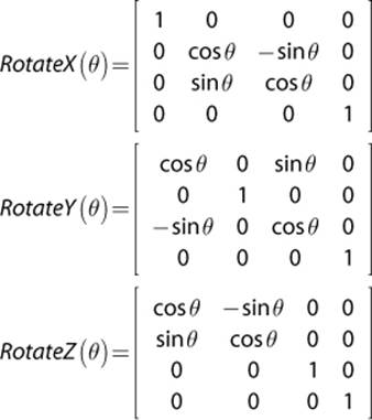
Rotation
A rotation matrix enables you to rotate a vector or position about a coordinate axis. There are three different rotation matrices, one for each Cartesian coordinate axis. So a rotation about the x-axis has a different matrix than a rotation about the y-axis. In all cases, the angle θ is passed into the matrix.
These rotations are known as Euler rotations, named after the Swiss mathematician.
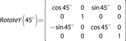
As an example, here is a matrix that rotates 45° about the y axis:
It can be somewhat daunting to remember these different rotation matrices. One trick that helps is to assign a number to each coordinate axis: x = 1, y = 2, and z = 3. This is because for the rotation about the x-axis, the element at (1,1) is 1, whereas everything else in the first row/ column is 0. Similarly, the y and z rotations have these values in the second and third row/column, respectively. The last row/column is always the same for all three matrices. Once you remember the location of the ones and zeros, the only thing left is to memorize the order of sine and cosine.
Rotation matrices are orthonormal, which means that the inverse of a rotation matrix is the transpose of that matrix.
Applying Multiple Transforms
It is often necessary to combine multiple transformations in order to get the desired world transform matrix. For example, if we want to position a character at a specific coordinate and have that character scale up by a factor of two, we need both a scale matrix and a translation matrix.
To combine the matrices, you simply multiply them together. The order in which you multiply them is extremely important, because matrix multiplication is not commutative. Generally, for the row-major representation, you want the world transform to be constructed as follows:
WorldTransform = Scale×Rotation×Translation
The rotation should be applied first because rotation matrices are about the origin. If you rotate first and then translate, the object will rotate about itself. However, if the translation is performed first, the object does not rotate about its own origin but instead about the world’s origin, as inFigure 4.3. This may be the desired behavior in some specific cases, but typically this is not the case for the world transform matrix.
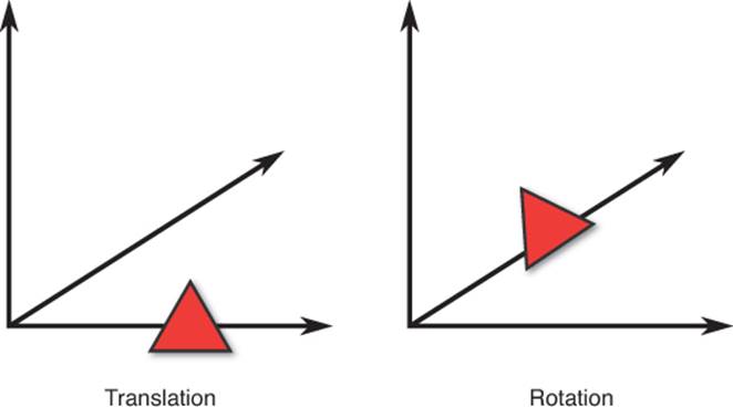
Figure 4.3 An object translated and then rotated about the world’s origin instead of about its own origin.
View/Camera Space
Once all the models are positioned and oriented in the world, the next thing to consider is the location of the camera. A scene or level could be entirely static, but if the position of the camera changes, it changes what is ultimately displayed onscreen. This is known as view or camera spaceand is demonstrated in Figure 4.4.
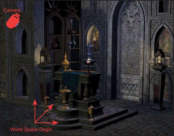
Figure 4.4 Camera space.
So we need another matrix that tells the graphics card how to transform the models from world space into a coordinate space that is relative to the camera. The matrix most commonly used for this is a look-at matrix. In a look-at matrix, the position of the camera is expressed in addition to the three coordinate axes of the camera.
For a row-major left-handed coordinate system, the look-at matrix is expressed as
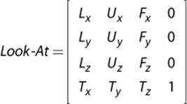
where L is the left or x-axis, U is the up or y-axis, F is the forward or z-axis, and T is the translation. In order to construct this matrix, these four vectors must first be calculated. Most 3D libraries provide a function that can automatically calculate the look-at matrix for you. But if you don’t have such a library, it’s not that hard to calculate manually.
Three inputs are needed to construct the look-at matrix: the eye, or the position of the camera, the position of the target the camera is looking at, and the up vector of the camera. Although in some cases the camera’s up vector will correspond to the world’s up vector, that’s not always the case. In any event, given these three inputs, it is possible to calculate the four vectors:
function CreateLookAt(Vector3 eye, Vector3 target, Vector3 Up)
Vector3 F = Normalize(target – eye)
Vector3 L = Normalize(CrossProduct(Up, F))
Vector3 U = CrossProduct(F, L)
Vector3 T
T.x = -DotProduct(L, eye)
T.y = -DotProduct(U, eye)
T.z = -DotProduct(F, eye)
// Create and return look-at matrix from F, L, U, and T
end
Once the view space matrix is applied, the entire world is now transformed to be shown through the eyes of the camera. However, it is still a 3D world that needs to be converted into 2D for display purposes.
Projection Space
Projection space, sometimes also referred to as screen space, is the coordinate space where the 3D scene gets flattened into a 2D one. A 3D scene can be flattened into 2D in several different ways, but the two most common are orthographic projection and perspective projection.
In an orthographic projection, the entire world is squeezed into a 2D image with no depth perception. This means that objects further away from the camera are the same size as objects closer to the camera. Any pure 2D game can be thought of as using an orthographic projection. However, some games that do convey 3D information, such as The Sims or Diablo III, also use orthographic projections. Figure 4.5 illustrates a 3D scene that’s rendered with an orthographic projection.
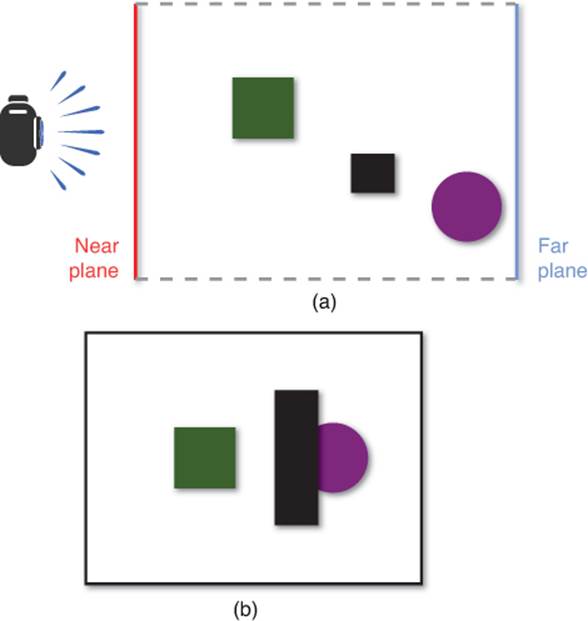
Figure 4.5 Top-down view of an orthographic projection (a), and the resulting 2D image onscreen (b).
The other type of projection commonly used is the perspective projection. In this projection, objects further away from the camera are smaller than closer ones. The majority of 3D games use this sort of projection. Figure 4.6 shows the 3D scene from Figure 4.5, except this time with a perspective projection.
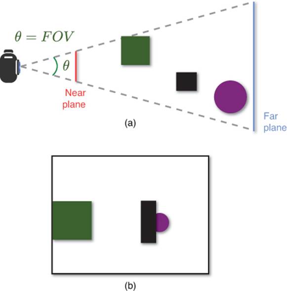
Figure 4.6 Top-down view of a perspective projection (a), and the resulting 2D image onscreen (b).
Both projections have a near and far plane. The near plane is typically very close to the camera, and anything between the camera and the near plane is not drawn. This is why games will sometimes have characters partially disappear if they get too close to the camera. Similarly, the far plane is far away from the camera, and anything past that plane is not drawn either. Games on PC will often let the user reduce the “draw distance” in order to speed up performance, and this often is just a matter of pulling in the far plane.
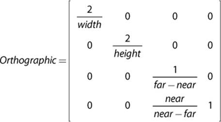
The orthographic projection matrix is composed of four parameters: the width and height of the view, and the shortest distance between the eye and the near/far planes:
The perspective projection has one more parameter, called field of view (FOV). This is the angle around the camera that is visible in the projection. Changing the field of view determines how much of the 3D world is visible, and is covered in more detail in Chapter 8, “Cameras.” Add in the FOV angle and it is possible to calculate the perspective matrix:
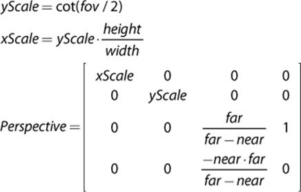
There is one last thing to consider with the perspective matrix. When a vertex is multiplied by a perspective matrix, its w-component will no longer be 1. The perspective divide takes each component of the transformed vertex and divides it by the w-component, so the w-component becomes 1 again. This process is actually what adds the sense of depth perception to the perspective transform.
Lighting and Shading
So far, this chapter has covered how the GPU is given a list of vertices as well as world transform, view, and projection matrices. With this information, it is possible to draw a black-and-white wireframe of the 3D scene into the 2D color buffer. But a wireframe is not very exciting. At a minimum, we want the triangles to be filled in, but modern 3D games also need color, textures, and lighting.
Color
The easiest way to represent color in a 3D scene is to use the RGB color space, which means there is a separate red, green, and blue color value. That’s because RGB directly corresponds to how a 2D monitor draws color images. Each pixel on the screen has separate red, green, and blue sub-pixels, which combine to create the final color for that pixel. If you look very closely at your computer screen, you should be able to make out these different colors.
Once RGB is selected, the next decision is the bit depth, or the number of bits allocated to each primary color. Today, the most common approach is 8 bits per color, which means there are 256 possible values each for red, green, and blue. This gives a total of approximately 16 million unique colors.
Because the range for the primary colors is 0 through 255, sometimes their values will be expressed in this manner. In web graphics, for instance, #ff0000 refers to 255 for red, 0 for green, and 0 for blue. But a more common approach in 3D graphics is to instead refer to the values as a floating point number between 0.0 and 1.0. So 1.0 is the maximum value for that primary color, whereas 0.0 is an absence of it.
Depending on the game, there is also the possibility of a fourth component, known as alpha. The alpha channel determines the transparency of a particular pixel. An alpha of 1.0 means that the pixel is 100% opaque, whereas an alpha of 0.0 means that it’s invisible. An alpha channel is required if the game needs to implement something like water—where there is some color the water gives off in addition to objects that are visible under the water.
So if a game supports full RGBA, and has 8 bits per component, it has a total of 32 bits (or 4 bytes) per pixel. This is a very common rendering mode for games. Figure 4.7 demonstrates a few different colors represented in the RGBA color space.
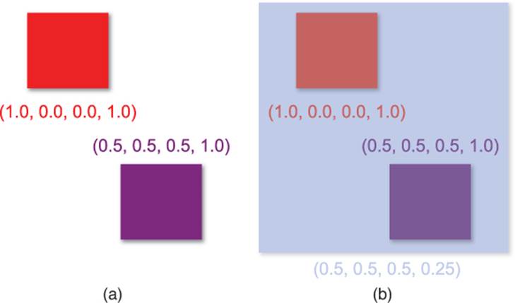
Figure 4.7 Opaque red and purple in the RGBA color space(a). A transparent blue allows other colors to be visible underneath (b).
Vertex Attributes
In order to apply color to a model, we need to store additional information for each vertex. This is known as a vertex attribute, and in most modern games several attributes are stored per each vertex. This, of course, adds to the memory overhead of the model and can potentially be a limiting factor when determining the maximum number of vertices a model can have.
A large number of parameters can be stored as vertex attributes. In texture mapping, a 2D image is mapped onto a 3D triangle. At each vertex, a texture coordinate specifies which part of the texture corresponds to that vertex, as demonstrated in Figure 4.8. The most common texture coordinates are UV coordinates, where the x-coordinate of the texture is named u and the y-coordinate of the texture is named v.
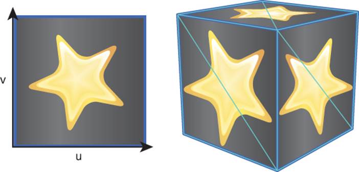
Figure 4.8 Texture mapping with UV coordinates.
Using just textures, it is possible to get a scene that looks colorful. But the problem is this scene does not look very realistic because there is no sense of light as there is in reality. Most lighting models rely on another type of vertex attribute: the vertex normal. Recall from Chapter 3, “Linear Algebra For Games,” that we can compute the normal to a triangle by using the cross product. But how can a vertex, which is just a single point, have a normal?
A vertex normal can be determined in a couple of different ways. One approach is to average the normals of all the triangles that contain that vertex, as in Figure 4.9(a). This works well if you want to have smooth models, but it won’t work properly when you want to have hard edges. For example, if you try to render a cube with averaged vertex normals, it will end up with rounded corners. To solve this problem, each of the cube’s eight corners must be represented as three different vertices, with each of the copies having a different vertex normal per face, as in Figure 4.9(b).
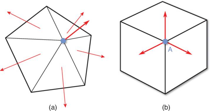
Figure 4.9 Averaged vertex normals (a). Vertex A on the cube uses one of three different normals, depending on the face (b).
Remember that a triangle technically has two normals, depending on the order in which the cross product is performed. For triangles, the order depends on the winding order, which can either be clockwise or counterclockwise. Suppose a triangle has the vertices A, B, and C in a clockwise winding order. This means that travelling from A to B to C will result in a clockwise motion, as in Figure 4.10(a). This also means that when you construct one vector from A to B, and one from B to C, the cross product between these vectors would point into the page in a right-handed coordinate system. The normal would point out of the page if instead A to B to C were counterclockwise, as in Figure 4.10(b). As with other things we’ve discussed, it doesn’t matter which winding order is selected as long as it’s consistent across the entire game.
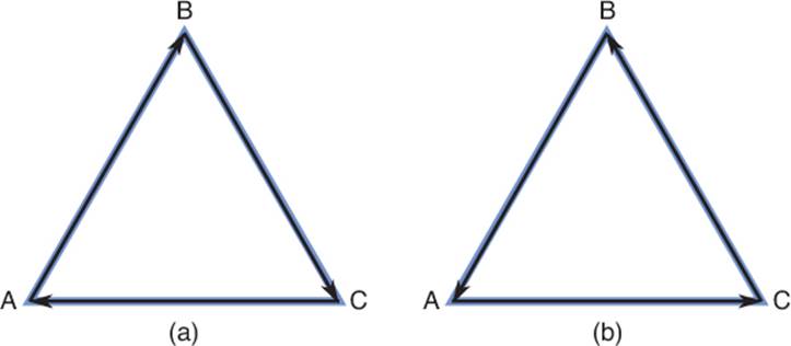
Figure 4.10 Clockwise winding order (a), and counterclockwise winding order (b).
One of the many things we might use to optimize rendering is back-face culling, which means triangles that are facing away from the camera are not rendered. So if you pass in triangles with the opposite winding order of what the graphics library expects, you may have forward-facing triangles disappear. An example of this is shown in Figure 4.11.
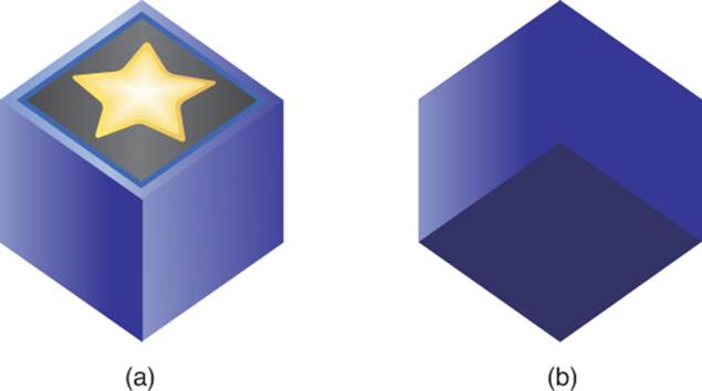
Figure 4.11 A cube rendered with the correct winding order (a), and the same cube rendered with the incorrect winding order (b).
Lights
A game without lighting looks very drab and dull, so most 3D games must implement some form of lighting. A few different types of lights are commonly used in 3D games; some lights globally affect the scene as a whole, whereas other lights only affect the area around the light.
Ambient Light
Ambient light is an uniform amount of light that is applied to every single object in the scene. The amount of ambient light may be set differently for different levels in the game, depending on the time of day. A level taking place at night will have a much darker and cooler ambient light than a level taking place during the day, which will be brighter and warmer.
Because it provides an even amount of lighting, ambient light does not light different sides of objects differently. So think of ambient light as the light outside on an overcast day when there is a base amount of light applied everywhere. Figure 4.12(a) shows such an overcast day in nature.

Figure 4.12 Examples in nature of ambient light (a) and directional light (b).
Directional Light
A directional light is a light without a position but that is emitted from a specific direction. Like ambient light, directional lights affect the entire scene. However, because directional lights come from a specific direction, they illuminate one side of objects while leaving the other side in darkness. An example of a directional light is the sun on a sunny day. The direction of the light would be a vector from the sun to the object, and the side facing the sun would be brighter. Figure 4.12(b) shows a directional light at Yellowstone National Park.
Games that use directional lights often only have one directional light for the level as a whole, representing either the sun or the moon, but this isn’t always a case. A level that takes place inside a dark cave may not have any directional lights, whereas a sports stadium at night might have multiple directional lights to represent the array of lights around the stadium.
Point Light
A point light is a light placed at a specific point that emanates in all directions. Because they emit from a specific point, point lights also will illuminate only one side of an object. In most cases we don’t want the point light to travel infinitely in all directions. For example, think of a light bulb in a dark room, as shown in Figure 4.13(a). There is visible light in the area immediately around the light, but it slowly falls off until there is no longer any more light. It doesn’t simply go on forever. In order to simulate this, we can add a falloff radius that determines how much the light decreases as the distance from the light increases.
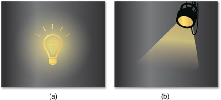
Figure 4.13 A light bulb in a dark room is an example of a point light (a). A spotlight on stage is an example of a spotlight (b).
Spotlight
A spotlight is much like a point light, except instead of travelling in all directions, it is focused in a cone. To facilitate the cone, it is necessary to have an angle as a parameter of spotlights. As with point lights, spotlights will also illuminate one side of an object. A classic example of a spotlight is a theater spotlight, but another example would be a flashlight in the dark. This is shown in Figure 4.13(b).
Phong Reflection Model
Once the lights have been placed in a level, the game needs to calculate how the lights affect the objects in the scene. These calculations can be done with a bidirectional reflectance distribution function (BRDF), which is just a fancy way of saying how the light bounces off surfaces. There are many different types of BRDFs, but we will only cover one of the most basic: the Phong reflection model. It should be noted that the Phong reflection model is not the same thing as Phong shading (which we will cover in a moment). The two are sometimes confused, but they are different concepts.
The Phong model is considered a local lighting model, because it doesn’t take into account secondary reflections of light. In other words, each object is lit as if it were the only object in the entire scene. In the physical world, if a red light is shone on a white wall, the red light will bounce and fill out the rest of the room with its red color. But this will not happen in a local lighting model.
In the Phong model, light is broken up into three distinctcomponents: ambient, diffuse, and specular, which are illustrated in Figure 4.14. All three components take into account both the color of the object and the color of the light affecting the object. The ambient component is tied to the overall illumination of the scene and can be directly tied to the ambient light. Because it’s evenly applied to the entire scene, the ambient component is independent of the location of lights and the camera.
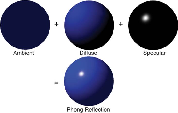
Figure 4.14 Phong reflection model.
The diffuse component is the primary reflection of light off the surface. This will be affected by any directional, point, or spotlights affecting the object. In order to calculate the diffuse component, you need the normal of the surface as well as a vector from the surface to the light. But as with the ambient component, the diffuse component is not affected by the position of the camera.
The final component is the specular component, which represents shiny highlights on the surface. An object with a high degree of specularity, such as a polished metal object, will have more highlights than something painted in matte black. As with the diffuse component, the specular component depends on the location of lights as well as the normal of the surface. But it also depends on the position of the camera, because highlights will change position based on the view vector.
Overall, the Phong reflection model calculations are not that complex. The model loops through every light in the scene that affects the surface and performs some calculations to determine the final color of the surface (see Listing 4.1).
Listing 4.1 Phong Reflection Model
// Vector3 N = normal of surface
// Vector3 eye = position of camera
// Vector3 pos = position on surface
// float a = specular power (shininess)
Vector3 V = Normalize(eye – pos) // FROM surface TO camera
Vector3 Phong = AmbientColor
foreach Light light in scene
if light affects surface
Vector3 L = Normalize(light.pos – pos) // FROM surface TO light
Phong += DiffuseColor * DotProduct(N, L)
Vector3 R = Normalize(Reflect(-L, N)) // Reflection of –L about N
Phong += SpecularColor * pow(DotProduct(R, V), a)
end
end
Shading
Separate from the reflection model is the idea of shading, or how the surface of a triangle is filled in. The most basic type of shading, flat shading, has one color applied to the entire triangle. With flat shading, the reflection model is calculated once per each triangle (usually at the center of the triangle), and this computed color is applied to the triangle. This works on a basic level but does not look particularly good.
Gouraud Shading
A slightly more complex form of shading is known as Gouraud shading. In this type of shading, the reflection model is calculated once per each vertex. This results in a different color potentially being computed for each vertex. The rest of the triangle is then filled by blending between the vertex colors. So, for example, if one vertex were red and one vertex were blue, the color between the two would slowly blend from red to blue.
Although Gouraud shading is a decent approximation, there are some issues. First of all, the quality of the shading directly correlates to the number of polygons in the model. With a low number of polygons, the shading may have quite a few hard edges, as shown in Figure 4.13(a). A high-polygon model can look good with Gouraud shading, but it’s at the additional memory cost of having more polygons.
Another issue is that smaller specular highlights often look fairly bad on low-polygon models, resulting in the banding seen in Figure 4.13(a). And the highlight may even be missed entirely if it’s so small that it’s contained only in the interior of a polygon, because we are only calculating the reflection model at each vertex. Although Gouraud shading was popular for many years, as GPUs have improved, it no longer sees much use.
Phong Shading
With Phong shading, the reflection model is calculated at every single pixel in the triangle. In order to accomplish this, the vertex normals are interpolated across the surface of the triangle. At every pixel, the result of the interpolation is then used as the normal for the lighting calculations.
As one might imagine, Phong shading is computationally much more expensive than Gouraud shading, especially in a scene with a large number of lights. However, most modern hardware can easily handle the increase in calculations. Phong shading can be considered a type of per-pixel lighting, because the light values are being calculated for every single pixel.
Figure 4.15 compares the results of shading an object with Gouraud shading and with Phong shading. As you can see, the Phong shading results in a much smoother and even shading.
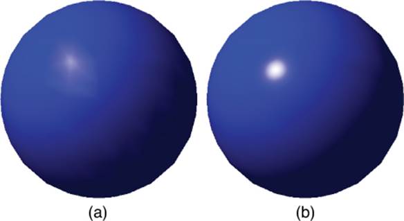
Figure 4.15 Object drawn with Gouraud shading (a), and an object drawn with Phong shading (b).
One interesting thing to note is that regardless of the shading method used, the silhouette is identical. So even if Phong shading is used, the outline can be a dead giveaway if an object is a low-polygon model.
Visibility
Once you have meshes, coordinate space matrices, lights, a reflection model, and shading, there is one last important aspect to consider for 3D rendering. Which objects are and are not visible? This problem ends up being far more complex for 3D games than it is for 2D games.
Painter’s Algorithm, Revisited
As discussed in Chapter 2, “2D Graphics,” the painter’s algorithm (drawing the scene back to front) works fairly well for 2D games. That’s because there’s typically a clear ordering of which 2D sprites are in front of each other, and often the 2D engine may seamlessly support the concept of layers. But for 3D games, this ordering is not nearly as static, because the camera can and will change its perspective of the scene.
This means that to use the painter’s algorithm in a 3D scene, all the triangles in the scene have to be resorted, potentially every frame, as the camera moves around in the scene. If there is a scene with 10,000 objects, this process of resorting the scene by depth every single frame would be computationally expensive.
That already sounds very inefficient, but it can get much worse. Consider a split-screen game where there are multiple views of the game world on the same screen. If player A and player B are facing each other, the back-to-front ordering is going to be different for each player. To solve this, we would either have to resort the scene multiple times per frame or have two different sorted containers in memory—neither of which are desirable solutions.
Another problem is that the painter’s algorithm can result in a massive amount of overdraw, which is writing to a particular pixel more than once per frame. If you consider the space scene from Figure 2.3 in Chapter 2, certain pixels may have been drawn four times during the frame: once for the star field, once for the moon, once for an asteroid, and once for the spaceship.
In modern 3D games, the process of calculating the final lighting and texturing for a particular pixel is one of the most expensive parts of the rendering pipeline. If a pixel gets overdrawn later, this means that any time spent drawing it was completely wasted. Due to the expense involved, most games try to eliminate as much overdraw as possible. That’s never going to happen with the painter’s algorithm.
And, finally, there is the issue of overlapping triangles. Take a look at the three triangles in Figure 4.16. Which one is the furthest back?
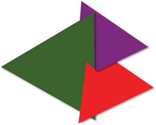
Figure 4.16 Overlapping triangles failure case.
The answer is that there is no one triangle that is furthest back. In this instance, the only way the painter’s algorithm would be able to draw these triangles properly is if some of them were split into multiple triangles.
Because of all these issues, the painter’s algorithm does not see much use in 3D games.
Z-Buffering
In z-buffering, an additional memory buffer is used during the rendering process. This extra buffer, known as the z-buffer, stores data for each pixel in the scene, much like the color buffer. But unlike the color buffer, which stores color information, the z-buffer (also known as the depth buffer) stores the distance from the camera, or depth, at that particular pixel. Collectively, the set of buffers we use to represent a frame (which can include a color buffer, z-buffer, stencil buffer, and so on) is called the frame buffer.
At the beginning of a frame rendered with z-buffering, the z-buffer is cleared out so that the depth at each pixel is set to infinity. Then, during rendering, before a pixel is drawn, the depth is computed at that pixel. If the depth at that pixel is less than the current depth value stored in the z-buffer, that pixel is drawn, and the new depth value is written into the z-buffer. A sample representation of the z-buffer is shown in Figure 4.17.
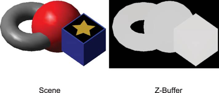
Figure 4.17 A sample scene and its corresponding z-buffer.
So the first object that’s drawn every frame will always have all of its pixels’ color and depth information written into the color and z-buffers, respectively. But when the second object is drawn, if it has any pixels that are further away from the existing pixels, those pixels will not be drawn. Pseudocode for this algorithm is provided in Listing 4.2.
Listing 4.2 Z-Buffering
// zBuffer[x][y] grabs depth at that pixel
foreach Object o in scene
foreach Pixel p in o
float depth = calculate depth at p
if zBuffer[p.x][p.y] > depth
draw p
zBuffer[p.x][p.y] = depth
end
end
end
With z-buffering, the scene can be drawn in any arbitrary order, and so long as there aren’t any objects with transparency, it will look correct. That’s not to say that the order is irrelevant—for example, if the scene is drawn back to front, you would overdraw a lot of pixels every frame, which would have a performance hit. And if the scene were drawn front to back, it would have no overdraw at all. But the idea behind z-buffering is that the scene does not need to be sorted in terms of depth, which can greatly improve performance. And because z-buffering works on a per-pixel basis, and not a per-object basis, it will work well even with the overlapping triangles case in Figure 4.16.
But that’s not to say z-buffering by itself solves all visibility problems. For one, transparent objects won’t work with z-buffering as is. Suppose there is semi-transparent water, and under this water there’s a rock. If pure z-buffering is used, drawing the water first would write to the z-buffer and would therefore prevent the rock from being drawn. To solve this issue, we first render all the opaque objects in the scene using normal z-buffering. Then we can disable depth buffer writes and render all the transparent objects, still checking the depth at each pixel to make sure we aren’t drawing transparent pixels that are behind opaque ones.
As with the representation of color, the z-buffer also has a fixed bit depth. The smallest size z-buffer that’s considered reasonable is a 16-bit one, but the reduced memory cost comes with some side effects. In z-fighting, two pixels from different objects are close to each other, but far away from the camera, flicker back and forth on alternating frames. That’s because the lack of accuracy of 16-bit floats causes pixel A to have a lower depth value than pixel B on frame 1, but then a higher depth value on frame 2. To help eliminate this issue most modern games will use a 24- or 32-bit depth buffer.
It’s also important to remember that z-buffering by itself cannot guarantee no pixel overdraw. If you happen to draw a pixel and later it turns out that pixel is not visible, any time spent drawing the first pixel will still be wasted. One solution to this problem is the z-buffer pre-pass, in which a separate depth rendering pass is done before the final lighting pass, but implementing this is beyond the scope of the book.
Keep in mind that z-buffering is testing on a pixel-by-pixel basis. So, for example, if there’s a tree that’s completely obscured by a building, z-buffering will still individually test each pixel of the tree to see whether or not that particular pixel is visible. To solve these sorts of problems, commercial games often use more complex culling or occlusion algorithms to eliminate entire objects that aren’t visible on a particular frame. Such algorithms include binary spatial partitioning (BSP), portals, and occlusion volumes, but are also well beyond the scope of this book.
World Transform, Revisited
Although this chapter has covered enough to successfully render a 3D scene, there are some outstanding issues with the world transform representation covered earlier in this chapter. The first problem is one of memory—if the translation, scale, and rotation must be modified independently, each matrix needs to be stored separately, which is 16 floating point values per matrix, for a total of 48 floating points for three matrices. It is easy enough to reduce the footprint of the translation and scale—simply store the translation as a 3D vector and the scale as a single float (assuming the game only supports uniform scales). Then these values can be converted to the corresponding matrices only at the last possible moment, when it’s time to compute the final world transform matrix. But what about the rotation?
There are some big issues with representing rotations using Euler angles, primarily because they’re not terribly flexible. Suppose a spaceship faces down the z-axis in model space. We want to rotate the space ship so it points instead toward an arbitrary object at position P. In order to perform this rotation with Euler angles, you need to determine the angles of rotation. But there isn’t one single cardinal axis the rotation can be performed about; it must be a combination of rotations. This is fairly difficult to calculate.
Another issue is that if a 90° Euler rotation is performed about a coordinate axis, the orientation of the other coordinate axes also changes. For example, if an object is rotated 90° about the z-axis, the x- and y-axes will become one and the same, and a degree of motion is lost. This is known asgimbal lock, as illustrated in Figure 4.18, and it can get very confusing very quickly.
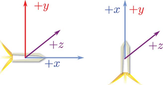
Figure 4.18 A 90° rotation about the z-axis causes gimbal lock.
Finally, there is a problem of smoothly interpolating between two orientations. Suppose a game has an arrow that points to the next objective. Once that objective is reached, the arrow should change to point to the subsequent one. But it shouldn’t just instantly snap to the new objective, because an instant change won’t look great. It should instead smoothly change its orientation, over the course of a second or two, so that it points at the new objective. Although this can be done with Euler angles, it can be difficult to make the interpolation look good.
Because of these limitations, using Euler angle rotations is typically not the preferred way to represent the rotation of objects in the world. Instead, a different math construct is used for this.
Quaternions
As described by mathematicians, quaternions are, quite frankly, extremely confusing. But for game programming, you really can just think of a quaternion as a way to represent a rotation about an arbitrary axis. So with a quaternion, you aren’t limited to rotations about x, y, and z. You can pick any axis you want and rotate around that axis.
Another advantage of quaternions is that two quaternions can easily be interpolated between. There are two types of interpolations: the standard lerp and the slerp, or spherical linear interpolation. Slerp is more accurate than lerp but may be a bit more expensive to calculate, depending on the system. But regardless of the interpolation type, the aforementioned objective arrow problem can easily be solved with quaternions.
Quaternions also only require four floating point values to store their information, which means memory is saved. So just as the position and uniform scale of an object can be stored as a 3D vector and float, respectively, the orientation of the object can be stored with a quaternion.
For all intents and purposes, games use unit quaternions, which, like unit vectors, are quaternions with a magnitude of one. A quaternion has both a vector and a scalar component and is often written as ![]() . The calculation of the vector and scalar components depends on the axis of rotation, â, and the angle of rotation, θ:
. The calculation of the vector and scalar components depends on the axis of rotation, â, and the angle of rotation, θ:
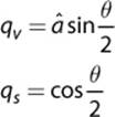
It should be noted that the axis of rotation must be normalized. If it isn’t, you may notice objects starting to stretch in non-uniform ways. If you start using quaternions, and objects are shearing in odd manners, it probably means somewhere a quaternion was created without a normalized axis.
Most 3D game math libraries should have quaternion functionality built in. For these libraries, a CreateFromAxisAngle or similar function will automatically construct the quaternion for you, given an axis and angle. Furthermore, some math libraries may use x, y, z, and w-components for their quaternions. In this case, the vector part of the quaternion is x, y, and z while the scalar part is w.
Now let’s think back to the spaceship problem. You have the initial facing of the ship down the z-axis, and the new facing can be calculated by constructing a vector from the ship to target position P. To determine the axis of rotation, you could take the cross product between the initial facing and the new facing. Also, the angle of rotation similarly can be determined by using the dot product. This leaves us with both the arbitrary axis and the angle of rotation, and a quaternion can be constructed from these.
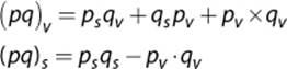
It is also possible to perform one quaternion rotation followed by another. In order to do so, the quaternions should be multiplied together, but in the reverse order. So if an object should be rotated by q and then by p, the multiplication is pq. The multiplication for two quaternions is performed using the Grassmann product:
Much like matrices, quaternions have an inverse. Luckily, to calculate the inverse of a unit quaternion you simply negate the vector component. This negation of the vector component is also known as the conjugate of the quaternion.
Because there is an inverse, there must be an identity quaternion. This is defined as:
Finally, because the GPU still expects the world transform matrix to be in matrix form, the quaternion will, at some point, need to be converted into a matrix. The calculation of a matrix from a quaternion is rather complex, so it’s not included in this text. But rest assured that your 3D math library most likely has a function to do this for you.
3D Game Object Representation
Once we are using quaternions, the translation, scale, and rotation can all be represented with data smaller than a single 4×4 matrix. This is what should be stored for the world transform of a 3D game object. Then, when it’s time to pass world transform matrix information to the rendering code, a temporary matrix can be constructed. This means that if code needs to update the position of the game object, it only needs to change the position vector, and not an entire matrix (see Listing 4.3).
Listing 4.3 3D Game Object
class 3DGameObject
Quaternion rotation
Vector3 position
float scale
function GetWorldTransform()
// Order matters! Scale, rotate, translate.
Matrix temp = CreateScale(scale) *
CreateFromQuaternion(rotation) *
CreateTranslation(position)
return temp
end
end
Summary
This chapter looked at many of the core aspects of 3D graphics. Coordinate spaces are an important concept that expresses models relative to the world and the camera, and also determines how we flatten a 3D scene into a 2D image. There are several different types of lights we might have in a scene, and we use BRDFs such as the Phong reflection model to determine how they affect objects in the scene. 3D engines also shy away from using the painter’s algorithm and instead use z-buffering to determine which pixels are visible. Finally, using quaternions is preferred as a rotation method over Euler angles.
There is much, much more to rendering than was covered in this chapter. Most games today use advanced rendering techniques such as normal mapping, shadows, global illumination, deferred rendering, and so on. If you are interested in studying more about rendering, there’s much to learn out there.
Review Questions
1. Why are triangles used to represent models in games?
2. Describe the four primary coordinate spaces in the rendering pipeline.
3. Create a world transform matrix that translates by ![]() 2, 4, 6
2, 4, 6![]() and rotates 90° about the z-axis.
and rotates 90° about the z-axis.
4. What is the difference between an orthographic and perspective projection?
5. What is the difference between ambient and directional light? Give an example of both.
6. Describe the three components of the Phong reflection model. Why is it considered a local lighting model?
7. What are the tradeoffs between Gouraud and Phong shading?
8. What are the issues with using the Painter’s algorithm in a 3D scene? How does z-buffering solve these issues?
9. Why are quaternions preferable to Euler angles for rotation representations?
10. Construct a quaternion that rotates about the x-axis by 90°.
Additional References
Akenine-Möller, Tomas, et. al. Real-Time Rendering (3rd Edition). Wellesley: AK Peters, 2008. This is considered the de facto reference for rendering programmers. Although this latest edition is a few years old now, it still is by far the best overview of rendering for games programmers.
Luna, Frank. Introduction to 3D Game Programming with DirectX 11. Dulles: Mercury Learning & Information, 2012. One thing about rendering books is they often focus on one specific API. So there are DirectX books and OpenGL books. Luna has written DirectX books since at least 2003, and when I was a budding game programmer I learned a great deal from one of his early books. So if you are planning on using DirectX for your game (remember that it’s PC only), I’d recommend this book.
All materials on the site are licensed Creative Commons Attribution-Sharealike 3.0 Unported CC BY-SA 3.0 & GNU Free Documentation License (GFDL)
If you are the copyright holder of any material contained on our site and intend to remove it, please contact our site administrator for approval.
© 2016-2026 All site design rights belong to S.Y.A.