Programming Elastic MapReduce (2014)

Chapter 5. Machine Learning Using EMR

So far we have covered various ways you can use EMR and AWS to accomplish some interesting tasks surrounding log data analysis. The next step in building such a system is to begin using machine learning algorithms aimed at predicting things based on your data. In the example for this chapter, we’ll use a clustering technique to derive interesting information about accesses to web log data.

A thorough discussion of machine learning is beyond the scope of this book. There are many great resources that will help you understand machine learning. Hilary Mason’s An Introduction to Machine Learning with Web Data is a great video course to get started. A more formal treatment of machine learning is available in this Coursera Machine Learning class. It’s taught by Stanford professor Andrew Ng and is very accessible to most people—you don’t need to be a computer scientist to learn the material.

This chapter will not make you a machine learning expert, but we present a few examples of how to use machine learning algorithms in EMR. Hopefully, this will pique your interest in learning more about this topic.

A Quick Tour of Machine Learning

What is machine learning? Put simply, machine learning is the application of statistical methods to derive meaning and understanding from information. The clustering algorithm we are going to use for this chapter is called k-Means. k-Means clustering is used to find a number of clusters, k, for a set of data. The exact number of clusters is user-defined—a bit more about this in a moment. The nice thing about k-Means is that you can have unlabeled data and derive meaning from it. This mode of machine learning is called unsupervised because no explicit labels or meaning is known ahead of time regarding the data.

As we just noted, k-Means is a clustering algorithm. This means it gathers points (your input data) around a predefined number of clusters, k. The idea is to help uncover clusters that occur in your data so you can investigate unusual or previously unknown patterns in your data.

The selection of the k clusters (or k-cluster centroids) is somewhat dependent on the data set you want to cluster. It is also part art and part science. You can start out with a small number, run the algorithm, look at the results, increase the number of clusters, rerun the algorithm, look at the results, and so on.

The other aspect of k-Means you need to be aware of is the distance measurement used. Once your data points and k-cluster centroids are placed in a space, generally Cartesian, one of several distance metrics is used to calculate the distance of each data point from a nearby centroid. The most common distance metric used is called Euclidean distance. Figure 5-1 shows the Euclidean formula for distance.

Euclidean formula

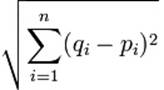
Figure 5-1. Euclidean formula

There are others distance metrics, which you can discover via one of the two resources listed at the beginning of this chapter.

The basic k-Means algorithm is as follows:

1. Take your input data and normalize it into a matrix of I items.

2. The k centroids now need to be placed (typically randomly) into a space composed of the I items.

3. A preselected distance metric is used to find the items in I that are closest to each of the k centroids.

4. Recalculate the centroids.

The iterative part of the algorithm is steps 3 and 4, which we keep executing until we reach convergence, which means the recalculations no longer produce change or the change is very minimal. At this point we execute the k-Means algorithm. Generally speaking, a concept called local minima is used to determine when convergence has occurred.

The example that is used in this chapter is based off sample code that Hilary Mason used in her Introduction to Machine Learning with Web Data video. The code she came up with takes a data file of delicious links and tags to generate a co-occurrence set of tags and URLs. A short snippet from the links file looks like this:

http://blog.urfix.com/25-%E2%80%93-sick-linux-commands/,"linux,bash"

http://sentiwordnet.isti.cnr.it/,"data,nlp,semantic"

http://www.pixelbeat.org/cmdline.html,"linux,tutorial,reference"

http://www.campaignmonitor.com/templates/,"email,html"

http://s4.io/,"streammining,dataanalysis"

http://en.wikipedia.org/wiki/Adolphe_Quetelet,"statistics,history"

The format basically is URL,[csv list of tags]. The co-occurrence is used to find similar things that occur close to each other. In the preceding data set, we are interested in knowing which URLs share the same tags.

NOTE

For those of you who want a more formal definition of co-occurrence, you can see its Wikipedia entry, which states: “Co-occurrence or cooccurrence is a linguistics term that can either mean concurrence/coincidence or, in a more specific sense, the above-chance frequent occurrence of two terms from a text corpus alongside each other in a certain order. Co-occurrence in this linguistic sense can be interpreted as an indicator of semantic proximity or an idiomatic expression.”

A nice property of the implementation is that not only are the tags clustered, but so are the URLs. An interesting extension of this k-Means implementation might be to take web server logs and cluster the geographic locations around common resources accessed on the web server(s). This idea has several interesting outcomes, including that it:

§ Helps you find what pages are more interesting to different parts of the US or world, thereby allowing you to tailor content appropriately

§ Helps you discover possible attacks from known cyberterrorism organizations that operate out of certain geographic locations

It is this idea that we will pursue in the coming section.

Python and EMR

Back in Chapter 3 we showed you how to use the elastic-mapreduce CLI tool. In this chapter, we will rely on this tool again, as opposed to the AWS user interface for running EMR jobs. This has several advantages, including:

§ It’s easy to use.

§ You can keep a number of EMR instances running for a period of time, thereby reducing your overall costs.

§ It greatly aids in debugging during the development phase.

Additionally, thus far in the book we have used Java programming examples. In this chapter we’ll use the Python programming language to show how you can use EMR to run machine learning algorithms.

NOTE

The mrjob Python framework allows you to write pure Python MapReduce applications. You can run the code on your local machine (which is great for debugging and testing), on a Hadoop cluster of your own, or on EMR. We are not going to use this tool for this chapter; we are going to use elastic-mapreduce, but just note that it’s out there for you to explore and use.

We’ll also use the s3cmd command-line tool to upload and retrieve code, data, and output files in S3.

Why Python?

So why use Python? Python has some great capabilities built into it for performing numerical computations. On top of this, the Pycluster Python library has some great support for performing k-Means clustering. This framework will be used to run the algorithm. Another nice thing about Python is that, similar to Perl, your development and deployment time are both greatly decreased because you can make code changes and immediately run your application to test or debug it.

NOTE

The scikit Python library implements many machine learning algorithms. It has great documentation and a ton of examples.

For the remainder of this section, we will discuss the data input for our application, the mapper code, and then the reducer code. Finally, we put it all together and show how to run the application on EMR.

The Input Data

Recall back in Chapter 2 where we had web log data that looked like this:

piweba2y.prodigy.com - - [02/Jul/1995:00:01:28 -0400] "GET ..." 404 -

dd04-014.compuserve.com - - [02/Jul/1995:00:01:28 -0400] "GET ..." 200 7074

j10.ptl5.jaring.my - - [02/Jul/1995:00:01:28 -0400] "GET ..." 304 0

198.104.162.38 - - [02/Jul/1995:00:01:28 -0400] "GET ..." 200 11853

buckbrgr.inmind.com - - [02/Jul/1995:00:01:29 -0400] "GET ..." 304 0

gilbert.nih.go.jp - - [02/Jul/1995:00:01:29 -0400] "GET ..." 200 1204

One of the things we can do is take the co-occurrence Python script and extend it to:

1. Look at the source of the web request.

2. Convert it to a geographic location.

3. Collect the resources accessed from this and other locations.

Note that in the web log data, the first field in the data is the source of the request.

An example data file might look like this:

path-to-resource,"csv list of geographic locations"

While we don’t show it in this chapter, there are open source and commercial geographic databases you can use to accomplish this task.

NOTE

MaxMind provides geolocation information for IP addresses. It has both web services and databases you can use. There are costs associated with using such a service, so be sure you understand exactly how you want to use something like this in your application.

The Mapper

Let’s take a look at the code for the mapper:

#!/usr/bin/env python

# encoding: utf-8

"""

tag_clustering.py

Created by Hilary Mason on 2011-02-18.

"""

import csv

import sys

import numpy

from Pycluster import *

class TagClustering(object):

def __init__(self):

self.load_link_data()

def load_link_data(self):

for line insys.stdin:

print line.rstrip()

if __name__ == '__main__':

t = TagClustering()

This mapper code is really just a shell and is meant for illustrative purposes. It reads the input fed to it on standard in stdin and spits it back out to standard out via stdout. This stdout is then read in by the reducer code—more on the reducer soon.

So what would a real-world mapper do? Here are the bits we’re leaving out:

§ It would handle parsing of the raw web log data to pull out the source hostname or IP address of the request.

§ It would do the geographic lookup for each source and group together resource access by geographic region. This step would be considered a postprocessing step.

§ Once done processing all raw log records, it would emit to standard out the resources and geolocations that will feed into the reducer.

Additionally, our example mapper only deals with a single input file. A real mapper is likely going to process multiple, large logfiles. So the input might actually be a directory containing the logfiles to process. The more data you have, especially over a long period of time (one month, two months, etc.), will greatly increase the results of the clustering process.

NOTE

If you pass an S3 directory (e.g., s3n://bucketname/files_to_process/) to the input option to EMR, it will handle taking all the files in the directory and divvying them up among multiple mapper jobs.

We’ve put together the following contrived postprocessed data for use in our application. Here is the sample:

"/history/apollo/","CA,TX"

"/shuttle/countdown/","AL,MA,FL,SC"

"/shuttle/missions/sts-73/mission-sts-73.html","SC,WA"

"/shuttle/countdown/liftoff.html","SC,NC,OK"

"/shuttle/missions/sts-73/sts-73-patch-small.gif","MS"

"/images/NASA-logosmall.gif","MS,FL"

"/shuttle/countdown/video/livevideo.gif","CO"

"/shuttle/countdown/countdown.html","AL"

"/","GA"

Basically what you have is a list of resources along with one or more geographic regions that accessed the resource. We’ve used US states, but you could also include country codes or other geo-identifiers.

The Reducer

The reducer code is presented next. The first thing you will notice is that it’s a little more involved than the mapper code. Areas that need more explanation are called out explicitly.

#!/usr/bin/env python

# encoding: utf-8

"""

tag_clustering.py

Created by Hilary Mason on 2011-02-18.

"""

import csv

import sys

import numpy

from Pycluster import *

class TagClustering(object):

def __init__(self):

tag_data = self.load_link_data()

all_tags = []

all_urls = []

for url,tags intag_data.items():

all_urls.append(url)

all_tags.extend(tags)

all_tags = list(set(all_tags)) # list of all tags in the space

numerical_data = [] # create vectors for each item

for url,tags intag_data.items():

v = []

for t inall_tags:

if t intags:

v.append(1)

else:

v.append(0)

numerical_data.append(tuple(v))

data = numpy.array(numerical_data)

# cluster the items

# 20 clusters, city block distance, 20 iterations

labels, error, nfound = kcluster(data, nclusters=6, dist='b',

npass=20)

# print out the clusters

clustered_urls = {}

clustered_tags = {}

i = 0

for url inall_urls:

clustered_urls.setdefault(labels[i], []).append(url)

clustered_tags.setdefault(labels[i], []).extend(tag_data[url])

i += 1

tag_list = {}

for cluster_id,tags inclustered_tags.items():

tag_list[cluster_id] = list(set(tags))

for cluster_id,urls inclustered_urls.items():

print tag_list[cluster_id]

print urls

def load_link_data(self):

data = {}

r = csv.reader(sys.stdin)

for row inr:

data[row[0]] = row[1].split(',')

return data

if __name__ == '__main__':

t = TagClustering()

The point of this code is to create a bit vector to feed into the clustering algorithm.

We must present the clustering algorithm with a vector. This code creates a numpy-formatted array. This representation is much more efficient than using the standard Python built-in array.

Here is where the heavy lifting is done. It makes a call into the Pycluster library function kcluster. Then it performs clustering based on how we configure it. In this example, we ask it to create 6 clusters, use the city-block distance measurement (dist=), and perform 20 passes (npass=). The number of passes tells kcluster how many times to pass through the data until the results converge, (i.e., there is little to no change in the calculations). Recall that the local minima will be used to determine convergence.

This code accumulates all of the clustered tags into a data structure. This acts as a lookup table when we print the clusters.

Using the lookup table of tags, the code prints out the states and the cluster of resources.

NOTE

The city-block distance measurement is also called the Manhattan distance, taxi cab distance, and others. You can read more about it here.

As note number 1 in the reducer code points out, a bit vector is used to encode the input data for presentation to the clustering algorithm. If you print the data array, it looks like this:

[[0 0 1 1 0 0 0 0 0 0 0 0]

[0 0 0 0 0 0 1 0 0 0 1 0]

[1 0 0 0 0 0 0 0 0 0 0 0]

[0 0 0 0 0 1 0 0 0 0 0 0]

[0 0 0 0 0 0 1 0 0 0 0 0]

[0 1 0 0 0 0 0 0 0 0 0 0]

[0 0 0 0 0 0 0 1 0 1 0 0]

[0 0 0 0 1 0 0 1 1 0 0 0]

[0 0 0 0 0 1 0 1 0 0 1 1]]

There is one row for each line of input from the data file. Each column represents the set of all geolocations (or tags, from the original implementation). This is I from our algorithm description earlier in the chapter. It is done this way because we are not initially starting with numerical data. Because we are clustering on nominal, text data, we must normalize the input data into a format consumable by the distance calculation we chose.

It should be noted that we are not taking into account the frequency of access to a given URL or resource. So if, for example, “/” were accessed a million times, we don’t care. Using logistic regression, we could predict the frequency with which a resource might get accessed in the future. TheAnalytics Made Skeezy blog has a great example on how to apply logistic regression (and how not to confuse it with linear regression).

NOTE

As you can imagine, the larger the data set you plan to vectorize, the more memory it will require. This might mean choosing larger instance types with more RAM and CPU power in your EMR cluster.

Putting It All Together

It’s now time to upload code and data files to S3 so you can provision the EMR cluster and run your MapReduce job. First, you need to get the Pycluster library installed onto your cluster. The reason you have to do this is because Pycluster is not available to Python on the EMR cluster by default. The way you accomplish this is by creating a script that downloads the tarball, extracts it, and runs the proper Python command to build and install the library. The script looks like this:

#!/bin/bash

# pycluster.sh

set -e

wget -S -T 10 -t 5 \

http://bonsai.hgc.jp/~mdehoon/software/cluster/Pycluster-1.52.tar.gz

mkdir -p ./Pycluster-1.52

tar zxvf Pycluster-1.52.tar.gz

cd Pycluster-1.52

sudo python setup.py install

Here, the sudo command is used to build and install Pycluster. Without using sudo, the library will be built and installed as the Hadoop user. You want to make sure the library gets installed to the normal location so your script can use it. Usage of the sudo command will not require password input, so it’s safe to use in this manner.

You are now ready to upload your input data, mapper code, reducer code, and pycluster.sh to S3:

$ s3cmd put links2.csv tag_clustering_mapper.py tag_cluster_reducer.py \

pycluster.sh s3://program-emr/

With all the parts in place, you can now turn up the EMR cluster. You will want to create the Job Flow and leave it alive for ease of rerunning the MapReduce application. The following command should hopefully be familiar to you:

$ elastic-mapreduce --create --enable-debug --alive \

--log-uri s3n://program-emr/emr/logs/ \

--instance-type m1.small \

--num-instances 1 \

--name python \

--bootstrap-action "s3://program-emr/pycluster.sh"

This is the bootstrap script you previously uploaded to S3. When AWS provisions an EMR cluster, this script is run. You can run up to 16 actions per elastic-mapreduce command. You can read more on bootstrap actions here.

Once the EMR cluster is bootstrapped and waiting for requests, you will have the Pycluster library installed and ready for use. This feature of EMR is a great way to get custom libraries and code on the cluster. This is also how you can alter various Hadoop options for the cluster.

You are now ready to run the MapReduce program. Start it with the following command:

$ elastic-mapreduce --stream \

--mapper s3://program-emr/tag_clustering_mapper.py \

--input s3://program-emr/links2.csv \

--output s3://program-emr/foo \

--reducer s3://program-emr/tag_clustering_reducer.py \

-j JOB_ID

You are specifying the --stream option to the elastic-mapreduce command. This means you also need to specify the path to the mapper, input data, output location, and reducer code. If you do not specify all four items, the stream command will fail.

This is the location where, upon success or failure, output will be placed.

This is the S3 path to your input data.

EMR will place success or failure status files in the S3 directory you specify with this option.

The reducer code you want EMR to run is passed to this option.

Once your MapReduce job is finished, you will want to make sure you terminate your cluster (recall we started it with the alive option):

$ elastic-mapreduce --terminate -j JOB_ID

Upon successful completion of the job, the reducer output will be placed in s3://program-emr/foo/part-00000. You can download this file for inspection with the following S3 command:

$ s3cmd get s3://program-emr/foo/part-00000

If your job failed for whatever reason, the files in the S3 directory will look like part-00001, part-00002, and so on. You can use these to determine why your job failed and go fix the issue.

If you open the part-00000 file in your favorite editor, you will see the following (note that the output was manually formatted to fit on the page):

['SC', 'WA']: ['/shuttle/missions/sts-73/mission-sts-73.html']

['CO', 'AL', 'GA']: ['/shuttle/countdown/video/livevideo.gif', \

'/shuttle/countdown/countdown.html', '/']

['SC', 'NC', 'OK']: ['/shuttle/countdown/liftoff.html']

['CA', 'TX']: ['/history/apollo/']

['SC', 'FL', 'MA', 'AL']: ['/shuttle/countdown/']

['FL', 'MS']: ['/images/NASA-logosmall.gif', \

'/shuttle/missions/sts-73/sts-73-patch-small.gif']

The output shows clusters around resources and the US states that tended to access them. Some of the clusters are straight out of the data file like that for SC and WA:

['SC', 'WA']: ['/shuttle/missions/sts-73/mission-sts-73.html']

But if you look at this line:

['FL', 'MS']: ['/images/NASA-logosmall.gif', \

'/shuttle/missions/sts-73/sts-73-patch-small.gif']

It is actually made up of these two data rows from our input file:

"/shuttle/missions/sts-73/sts-73-patch-small.gif","MS"

"/images/NASA-logosmall.gif","MS,FL"

The results are not perfect. You can see that another FL from our input file appears in this output line:

['SC', 'FL', 'MA', 'AL']: ['/shuttle/countdown/']

Recall that k-Means uses local minima to determine when it has converged. This can cause poor clusters to be formed, which can cause the results to be suboptimal. The bisecting k-Means algorithm is an extension on k-Means that aims to deal with poor cluster creation. The hierarchical clustering is yet another algorithm that can help overcome poor convergence.

What About Java?

The Mahout Java library implements many popular machine learning algorithms with an eye toward running on Hadoop. You can download the source package, build it, and run prepackaged examples. Running Mahout in EMR is also possible, with a bit of work.

What’s Next?

This chapter showed the basics of how you can use EMR to run machine learning algorithms. Something worth noting is that not all data sets are amenable to running on Hadoop, especially if splitting up the data set at map time will introduce inconsistencies in the final results. This is also true of machine learning algorithms—not all of them play nicely with the MapReduce paradigm.

For the curious-minded folks, here are three easy steps to becoming a machine learning expert:

§ Learn all you can about different machine learning algorithms, including the math behind them.

§ Experiment with sample code so you can take theory and turn it into practice.

§ Once you are familiar with machine learning, you can start thinking about your particular domain and how you can apply these algorithms to your data.