Professional Embedded ARM Development (2014)
Part I. ARM Systems and Development
Chapter 10. Writing Optimized C
WHAT’S IN THIS CHAPTER?
Knowing when to optimize
Knowing what to optimize
C optimization techniques
Assembly optimization techniques
Hardware optimization
Optimization is the final part of any project, and it is vitally important to understand. Some developers write optimized code from the start, and on most projects, that is a bad idea. The reason is simple: Optimized code is often difficult to read or to understand, and during the development phase, changes have to be made, often from different people, and in some cases, different departments. It is often best to start with readable, maintainable code before starting the optimization process. In addition, spending an extra two hours on optimizing a section of code might not be worth it; maybe this function will be called only once, or maybe the entire file will be replaced when changes occur in the project.
When the project is finished, when all the functionality has been added and all the bugs have been corrected, now it’s time to start optimizing. The problem is, where do you start?
RULES FOR OPTIMIZED CODE
The term rules are used, but the truth is there are no set rules. You do not need to follow every rule here, indeed, for some applications; some of these rules might be impractical. You are the only judge as to what should be used and what shouldn’t. The previous code used 32-bit integers, but in some cases, you would prefer (or need) to have two 16-bit numbers because space could be critical, and the need for space-saving techniques supersedes the need to optimize for speed.
Don’t Start with Optimization
This might sound like a contradiction, but it is also one of the most important unwritten rules. Optimized code of course makes an application or system run faster, but it can make the code less readable. It is also easier to make mistakes in optimized code, simply because the code, being written specifically for a processor, is sometimes written in a less logical manner for humans. Also, is the code that you write going to be used often? It is suggested for most code to write clean code, not necessarily writing heavy optimizations or wasting cycles. The most important part of a project is to get the foundations ready and to get the basic structure. After the project works, then comes the time for optimization.
Like most rules, there are exceptions. One of them concerns interrupt handlers. Interrupts can play a critical role in development and need to be taken care of quickly. On a device that handles multiple interrupts, even during the development phase, handlers need to be at least slightly optimized, and any code that runs in an interrupt context needs to be fast.
Know Your Compiler
The first rule: Know your compiler. A compiler, without any instructions, normally creates a binary that can be used for debugging, but rarely anything optimized. To get the compiler to optimize for speed or size, normally you have to add compiler options. A compiler can be configured to optimize for size, or for speed, or a mixture of both. It can also be configured to not optimize at all, which is useful for debugging.
This is far beyond the scope of this book (and is a subject large enough to merit a book of its own). If your project requires optimized code, you should look closely at ARM’s compiler. ARM’s compiler contains some of the most advanced optimization routines available, designed by the people who designed the core.
Know Your Code
Again, this sounds like a contradiction. Of course, you know the code; after all, you wrote it, but how many times is your function actually called? How long does this routine take to execute? Knowing the answer to these two questions can also answer another question. What should you optimize? Shaving off 200 milliseconds might be a good optimization, but if that portion of code is run only once, the time spent optimizing might have been wasted. Saving a single millisecond on a routine that is called thousands of times, on the other hand, might have a huge impact.
PROFILING
In software engineering, profiling is a form of dynamic program analysis that measures, for example, the amount of memory used or the time a program takes to complete the usage of particular instructions or the frequency and duration of function calls. Using a profiler, you can get a good idea of what your code is doing, which portions of code are called frequently, and most important, the amount of times that certain routines take.
The trouble with embedded systems is that they are so different. What might work well on one embedded system might not work on another. Some systems will have an operating system, others will be bare-metal.
Profiling Inside an Operating System
Profiling on an embedded system with an operating system (especially the Cortex-A line) is relatively easy. For example, on Linux-based systems, GNU’s gprof is an excellent tool to use, but using such a tool requires several things to be present (disk space, for one).
To prepare a program to be profiled via gprof, it must be compiled with a special option, telling the compiler to add little bits of code to your own. To compile for profiling, simply add the -pg option:
arm-none-linux-gcc -o myprog myprog.c utils.c -g -pg
By adding this option, calls are added to monitor functions before each function call. This is used for creating statistical data about which function was run, how many times, and the amount of time spent.
After the program is compiled for profiling, it must be run to generate the information that gprof needs. Simply run the program as you would normally, using the same command-line options, and the program will run and create the necessary data files. The program will run slightly slower because debug routines have been added, but it shouldn’t be noticeable.
When the program has completed, it’s time to use gprof, which requires two files: the output file that was created, and the executable file itself. If you omit the executable filename, the file a.out is used. If you give no profile data filename, the file gmon.out is used. If any file is not in the proper format, or if the profile data file does not appear to belong to the executable file, an error message prints.
Gprof can output statistical data to an output file for analysis.
Flat profile:
Each sample counts as 0.001 seconds.
% cumulative self self total
time seconds seconds calls ms/call ms/call name
80.24 5.84 5.120 4000 1.28 1.28 calcfreq
20.26 1.45 1.280 4000 0.32 0.32 getio
00.00 0.01 0.009 1 8.96 8.96 precalc
This example printout shows a program that was run with the GNU profiler. This program is designed to get data from a GPIO and then calculate the frequency of the input signal. There are three functions: calcfreq, getio, and precalc. calcfreq takes (on average) 1.28 ms to execute andgetio only 0.32, but precalc takes a whopping 8.96 ms. At first, it is tempting to optimize the function that takes the most time, but have a closer look. precalc is called only once, but calcfreq, which takes only one-eighth of the time to run, is called 4,000 times. If optimization is required, this is the function to optimize because saving even one-tenth of a millisecond in this function results in a savings of more than the precalc function itself.
Profilers like this work by analyzing the program’s program counter at regular intervals. It requires operating system interrupts, and as such, cannot be used on barebones systems. It also gets its data by statistical approximation, so the results are not accurate, but they are precise enough to give you a general idea.
For Linux systems, oprofile is an excellent tool. This tool, released under the GNU GPL, leverages the hardware performance counters of the CPU to enable profiling for a wide variety of statistics. No special recompilations are required, and even debug symbols are not always necessary. It can be used to profile a single application, or it can be used to profile the entire system.
Profiling on a Bare Metal System
Profiling on a bare metal system is slightly more complicated because often there isn’t an operating system running that enables OS interrupts. There are, however, other options.
Hardware Profiler
As shown in the previous chapter, you can connect hardware devices to development boards for debugging. Some of these devices use the same interface for more advanced functions, including profiling.
Hardware profilers are more accurate than software profilers and have the advantage of not modifying code. The company Segger (http://www.segger.com) develops JTAG emulators for ARM systems, called the J-Link, which can be used to profile applications. Lauterbach Trace32 systems also have advanced profiling solutions. The DS-5 debugger from ARM is also a professional solution, offering advanced features.
Some manufacturers provide debugging interfaces directly onto evaluation boards, something that is important for the first steps of development.
For example, Silicon Labs provides evaluation boards equipped with J-Link technology. These boards not only give information about the routines being run, but they also correlate the amount of energy that each routine uses. Because Silicon Labs EFM32 series are heavily focused on energy efficiency, its tools also show some advanced statistics on energy usage. For example, when profiling an application, you can tell not only how often a particular routine is called, but also the amount of energy that it uses. This greatly helps specific profiling; optimization will not only be for the amount of time a routine takes, but also the amount of energy, which is an embedded engineer’s biggest dilemma. This solution provides the tools required to fully understand what portions of code require optimization, and what type.
Silicon Labs energyAware Profiler shows a real-time graph of power consumption, and with all the points of interest. It is possible to see that IRQ awoke the microcontroller, the event that returned it to sleep mode, the functions run, and the amount of CPU time for each routine. Of course, there is also an external debug port if you want to use your own tools.
GPIO Output
Another technique that you can use to profile specific functions is an available GPIO line. With the help of an oscilloscope, it is easy to see exactly how much time a routine takes.
For example, imagine an interrupt function on a Cortex-M microcontroller. Some Cortex-M devices have fast I/O capable of switching in two cycles or less. This is perfect for such a routine. At the beginning of the interrupt, set the I/O to a logical 1. At the end of the routine, switch the I/O back to a logical 0. On the oscilloscope, set a trigger on the output, and you can see exactly how long each routine or each specific event takes. You aren’t tied to an entire routine, but just about any section of code.
Cycle Counter
Some ARM cores have a Performance Monitor Unit, a small unit that can be programmed to gather statistics on the operation of the processor and memory system. In this case, you can use it to calculate the number of cycles a portion of code takes.
You can access the Performance Monitor Unit through the CP15 coprocessor, which is available on select cores. Because you access it through CP15, it requires system privileges, and thus can be programmed only by the kernel or through privileged code. By default, the counters are disabled. First, user-mode access to the performance counter must be enabled.
/* enable user-mode access to the performance counter*/
asm ("MCR p15, 0, %0, C9, C14, 0\n\t" :: "r"(1));
When this command is issued, the cycle counter starts incrementing. The cycle counter can then be read in user space, with a simple command:
static inline unsigned int get_cyclecount (void)
{
unsigned int cycles;
// Read CCNT Register
asm volatile ("MRC p15, 0, %0, c9, c13, 0\t\n": "=r"(cycles));
return cycles;
}
You can use this counter by comparing the number of cycles before and after the code section, or reset it as required. Also, for long routines, it has a divider, which can increment once every 64 cycles.
static inline void init_perfcounters (int32_t do_reset, int32_t enable_divider)
{
// in general enable all counters (including cycle counter)
int32_t value = 1;
// peform reset:
if (do_reset)
{
value |= 2; // reset all counters to zero.
value |= 4; // reset cycle counter to zero.
}
if (enable_divider)
value |= 8; // enable "by 64" divider for CCNT.
value |= 16;
// program the performance-counter control-register:
asm volatile ("MCR p15, 0, %0, c9, c12, 0\t\n" :: "r"(value));
// enable all counters:
asm volatile ("MCR p15, 0, %0, c9, c12, 1\t\n" :: "r"(0x8000000f));
// clear overflows:
asm volatile ("MCR p15, 0, %0, c9, c12, 3\t\n" :: "r"(0x8000000f));
}
C OPTIMIZATIONS
Although assembly language gives you full control over the processor, it isn’t practical to write large portions of software in assembly. For embedded projects, most engineers prefer C. C is portable, is much easier to write and maintain than assembly, and yet can still make highly optimized code. However, again, there is a difference between application development and embedded development. There are a few rules to follow, and to fully understand what is going on, you need to know about what the compiler is doing and the assembly it generates.
Basic Example
Start with a simple program.
void loopit(void)
{
u16 i; //Internal variable
iGlobal = 0; //Global variable
//16 bit index incrementation
for (i = 0; i < 16: i++)
{
iGlobal++;
}
}
This is an extremely simple program; it creates a loop that runs 16 times, each time incrementing a global variable. The code was compiled, transferred, and then run with a debugger capable of advanced performance monitoring. The application code comes in at 24 bytes, and on an ARM926EJ-S evaluation board, it runs in 138 μs. Most people would think that is great, but embedded engineers go pale with this. There is nothing strictly wrong with the code; it is perfectly good C code, highly maintainable, but there are things that can be done to make it run faster. ARM systems, and indeed a lot of systems, actually do better when they count down to zero. The reason is simple; every time the processor makes a calculation, the processor automatically compares it to zero and sets a processor flag. On this platform, the bit in question is Z in the CPSR register. At the end of each loop, i is compared to an integer. If you decreased to zero, you could add a jump condition if Z is true, saving cycles. So, make a quick change, and count down to zero:
void loopit(void)
{
u16 i; //Internal variable
//16 bit index decrementation
for (i = 16; i != 0: i--)
{
iGlobal++;
}
}
The size of the code remains unchanged; you are still at 24 bytes, but the execution time is faster, 124 μs. That is a bit of a speed gain, but there is still a lot you can do. The code uses a variable that is 16 bits long, presumably to save space. The loop can loop only 16 times, so why bother having a 32-bit variable? 16 should do. Actually, it does, but it isn’t always a good idea. This particular ARM core is 32-bit native, and using 16-bit values takes up valuable processor power because the processor has to convert a 16-bit variable to 32 bits, work with it, and then retransform it to 16 bits. Working with the native size can help. So turn that into a 32-bit variable:
void loopit(void)
{
u32 i; //Internal variable
iGlobal = 0; //Global variable
//32 bit index decrementation
for (i = 16; i != 0: i--)
{
iGlobal++;
}
}
Now, when debugging, you notice something. The size has gone down to 20 bytes because there are fewer instructions needed. Execution time has also gone down to 115 μs, again, because there are fewer instructions to execute. The joys of optimizing! But you aren’t done yet. That global variable is a nightmare; every time you loop, the processor needs to access the RAM to change a variable, and that uses up valuable time. So, now define a variable, keep it local, and at the end of the loop, copy it back to the global variable:
void loopit(void)
{
u32 i; //Internal variable
u32 j;
iGlobal = 0; //Global variable
//32 bit index decrementation
for (i = 16; i != 0: i--)
{
j++;
}
iGlobal = j; //Copy the local variable's value to the global variable
}
You haven’t done a lot here; all you have done is to declare a new variable and use that for the loop instead. Again, there is no size change; there are new codes for accessing a register, but you don’t have the codes to access RAM. Because the variable is now in a register, it is a considerable speed boost; the execution time is now down to 52 μs. But you can still do better. The loop creates a lot of overhead, and where possible, unrolling a loop can help:
void loopit(void)
{
u32 i; //Internal variable
u32 j;
iGlobal = 0; //Global variable
//32 bit index decrementation
for (i = 4; i != 0: i--)
{
j++; j++; j++; j++;
}
iGlobal = j; //Copy the local variable's value to the global variable
}
This time, you loop only 4 times, instead of 12, and doing 4 times the work inside the loop. This might sound strange, but this saves considerable overhead time; looping and forking take up valuable cycles. With this new routine, the size has gone up slightly to 22 bytes, but the execution time is down to 26 μs. There wasn’t anything wrong with the code, but there are always ways to optimize, and time should be taken for code optimization, especially on embedded systems. That isn’t an excuse for not being careful on powerful platforms; just because processors go faster and faster, it isn’t a reason to use up valuable cycles.
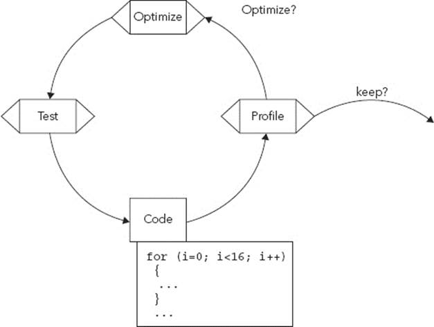
In total, optimization saved 112μs, a reduction of 81 percent. However, to achieve this result, several optimization cycles were performed. The code was profiled, then optimized, and then tested, repeating the cycle. Optimization can be a long procedure, testing multiple theories, possibly keeping the results, or reverting to the previous configuration. The cycle is illustrated in Figure 10-1.
FIGURE 10-1: Optimization cycle
Count Down, Not Up
It’s common to see code counting up, but as far as the processor is concerned, it is faster to count down to zero. To fully understand why, you need to look at the assembly code.
When you start the for loop, you initialize one of the registers to zero. Then you do the calculation, or break to another portion of code. At this point, increment the register. Compare the register to another number, and this takes up one cycle. If the result is lower, return to the beginning of the loop.
MOV r0, 0 @The amount of loops we have done
loop:
[ ... ]
ADD r0, r0, #1 @ Add one
CMP r0, #15
BLE loop
If you start at a certain number and count down to zero, things are slightly different. Initialize one of the registers to the number you want. Then, again, do the calculation or break to another portion of code. Here, you can decrement the register and force a status update. In the previous code, you would have compared the register to another number, but you don’t need to here. The CPSR would have been updated, so instead of comparing, you can simply Branch if Not Equal.
MOV r0, 16 @The amount of loops left to do
loop:
[ ... ]
SUBS r0, r0, #1 @ Subtract one
BNE loop
As you can see, you no longer have the CMP instruction. You have just saved a cycle per iteration. Not the most drastic speed-up possible, but if a routine has to loop thousands of times, it starts to build up.
Integers
Integers are a vital part of any development. Processors were designed to handle integers, not floating point or any other type of numeral. Ever since their introduction, special instructions or coprocessors for handling floating point numbers have been added on select cores, but despite optimization and engineering, they take longer to execute than integer arithmetic. You invariably use integers for standard calculation.
Most integer operations can be done in just a few cycles, with one notable exception, division, discussed in the next section. Generally, always use integers that are the same width as the system bus to avoid unwanted calculations later. Although a u16 might be all you need to hold in the data, if the variable is heavily used on a 32-bit system, making it a u32 can speed things up. When reading in a u16, the processor invariably reads in a u32 and then does some operations to transform it into a u16, which costs cycles.
Also, if you know that your variable can handle only positive numbers, make it unsigned. Most processors can handle unsigned integer arithmetic considerably faster than signed. (This is also good practice and helps make for self-documenting code.) Always try to make your code use integers. If you need two decimal places, multiply your figures by 100 instead of using a floating point.
Division
In the early days of ARM processors, ARM studied the needs for their processor carefully, and made a choice to not integrate a hardware division unit. This made the processor simpler, cheaper, and faster. Divisions were not all too common, and the divisions that were required could still be performed in software using highly optimized routines.
Division is complicated and requires a substantial number of transistors to be performed quickly. Some ARM processors have hardware division integrated, but some do not. Hardware division (present on Cortex-M3, Cortex-M4, and Cortex-A15/Cortex-A7 cores to name but a few) takes between 2 and 12 cycles.
General rule: If you can avoid dividing, avoid it. A 32-bit division in software can take up to (and in some cases more than) 120 cycles.
Sometimes you can get away with multiplying instead of dividing, especially when comparing. (a / b) > c can sometimes be rewritten as a > (c * b).
You can use shifting, although not technically dividing, as division. Where possible, the compiler attempts to shift rather than divide, but that works only for few cases. If the compiler cannot shift, it falls back to software routines for division.
Knowing what is required is essential to optimization. For example, if a program often divides by 10, you can write a small function that multiplies a number by 3277 and then divides the result by 32768.
add r1, r0, r0, lsl #1
add r0, r0, r1, lsl #2
add r0, r0, r1, lsl #6
add r0, r0, r1, lsl #10
mov r0, r0, lsr #15
This function does have a limited range, and care must be taken to ensure that the multiplication does not overflow. In some cases this can also be an approximation, not an exact result, but it is an example of what you can do by carefully rethinking routines to change them into shifts. In certain circumstances, when the maximum value of a variable is known, dividing in this fashion can save cycles.
Don’t Use Too Many Parameters
When writing C code, some developers are tempted to use large functions with multiple parameters. Some coding conventions call for small routines to be used, no longer than a printed page in length, but go into little detail about the parameters.
When you call a function in C, generally this is translated as a branch in assembly. The standard ARM calling convention dictates that parameters are passed by placing the parameter values into registers r0 through r3 before calling the subroutine. This means that a C routine typically uses up to four 32-bit integers as parameters, and any other parameters will be put onto the stack. You could just use higher registers, putting parameters into r4, r5, and so on, but at some point, something must be decided, and ARM chose this to be its calling convention. If you design a small assembly program, you can do anything you want, but a compiler sticks to the rules to simplify things.
Compilers can be configured to use a certain number of registers before pushing further variables onto the stack.
The ARM calling convention states that r0 to r3 are used as parameters for functions (r0 is also used as a return variable), and r4 to r12 are caller-save, meaning that a subroutine must not modify the value on return. A subroutine may of course modify any registers, but on return, the contents must have been restored. To do this, the subroutines must push the registers it needs to the stack and then pop them on return.
Pointers, Not Objects
When a subroutine is called, the first four parameters are passed as registers; all the others are pushed onto the stack. If a parameter is too big, it is also pushed onto the stack. Calling a subroutine by giving it a table of 64 integers can create considerably more overhead than giving it one parameter, the address of the table. By giving our subroutine the address of the object, you no longer need to push anything onto the stack, saving time and memory. The routine can then fetch the data with the memory address, and it is quite possible that only a few elements are required, not the entire table.
Don’t Frequently Update System Memory
In the previous example, you updated a global variable. When updating a global variable, or any variable that is not enclosed in your subroutine, the processor must write that variable out to system memory, waiting for the pipeline. In the best case, you get a cache hit, and the information will be written fairly quickly, but some zones are non-cacheable, so the information needs to be written out to system memory. Keeping a local variable in your subroutine means that in the best case, you update a register, keeping things extremely fast. After your routine finishes, you can write that value back out to system memory, incurring a pipeline delay only once.
Be careful when doing this, however, to make sure that you can keep a local copy in register memory. Remember that an interrupt breaks the current process, and your interrupt might need the real value. Also, in threaded applications, another thread may need the variable, in which case the data needs to be protected before writing (and frequently before reading, too).
This is one of the optimizations that can drastically improve performance, but great care must be taken.
Alignment
Alignment is vitally important in ARM-based systems. All ARM instructions must be aligned on a 32-bit boundary. NEON instructions are also 32-bits long, and must be aligned similarly. Thumb instructions are different and can be aligned on a 16-bit boundary. If instructions are to be injected from an external source (data cartridge, memory card, and so on), great care must be taken to put the data in the right location, since misaligned instructions will be interpreted as an undefined instruction.
Data alignment is a little different. Although it is advisable to use data that has the same width as the system bus, sometimes this isn’t possible. Sometimes, data needs to be packed, such as hardware addresses, network packets, and so on. ARM cores are good at fetching 32-bit values, but in a packet structure, an integer could be on a boundary between two double words. In the best case, this requires multiple instructions to fetch the memory and by using shifts, get the final result. In the worst case, it can result in an alignment trap, when the CPU tries to perform a memory access on an unaligned address.
ASSEMBLY OPTIMIZATIONS
When C optimizations are not enough, sometimes it is necessary to go a step further and look at assembly. Normally the compiler will do an excellent job in translating C to assembly, but it cannot know exactly what you want to do, and the scope of the action requested. Sometimes the compiler needs a hand, and sometimes you have to write short routines.
Specialized Routines
C compilers have to take your functions and translate them into assembly, without knowing all the possible use cases. For example, a multiplication routine might have to automatically take any number (16-bit, 32-bit, or maybe even 64-bit) and multiply that with any other combination. The list is endless. In most cases, there will be only a few use cases. For example, in an accounting program, maybe the only division possible will be dividing by 100, converting a number in cents to a number in dollars.
In embedded systems, it is often useful to create highly optimized routines for specific functions, mainly mathematical operations. For example, a quick routine for multiplying a number by 10 could be written as follows, taking only two cycles to complete.
MOV r1, r0, asl #3 ; Multiply r0 by 8
ADD r0, r1, r0, asl #1 ; Add r0 times 2 to the result
Don’t hesitate to create several routines like this in a helper file. In some cases, optimized libraries are available for use.
Handling Interrupts
Interrupts are events that force the processor to stop its normal operation and respond to another event. Interrupt handlers should be designed to be as fast as possible, signaling the interrupt to the main program through a flag or system variable before returning to the main application. The kernel (if available) can reschedule the applications to take into account an interrupt; if an interrupt handler is given the task of calculation, or any other routine that takes a long time, other interrupts might have to wait for the first interrupt to finish, resulting in surprising results.
For critical interrupts, FIQ is available. FIQ has a higher priority than IRQ, and on ARMv7A/R cores, the FIQ vector is at the end of the vector table, meaning that it is not necessary to jump to another portion of memory. The advantage is that this saves a branch instruction and also saves a potential memory reread. On most systems, the memory located at 0x00000000 is internal memory and doesn’t suffer from the same latency as external memory.
Interrupt Handling Schemes
There are several ways to handle interrupt, all depending on the project. Each has its own advantage and disadvantage, and choosing the right scheme is important for any project.
A non-nested interrupt handler handles interrupts sequentially.
A nested interrupt handler handles multiple interrupts, last in first out.
A re-entrant interrupt handler handles multiple interrupts and prioritizes them.
On a system with few interrupts, a non-nested handler is often enough and can be easily made to be extremely fast. Other projects handling lots of interrupts may need a nested handler, and projects with interrupts coming from multiple sources might require a re-entrant interrupt handler.
Non-Nested Interrupt Handler
The simplest interrupt handler is the non-nested interrupt handler. When entering this handler, all interrupts are disabled, and then the interrupt handler handles the incoming request. When the interrupt handler has completed its task, interrupts are re-enabled, and control is returned to the main application.
Nested Interrupt Handler
The nested interrupt handler is an improvement over the non-nested handler; it re-enables interrupts before the handler has fully serviced the current interrupt. Mainly used on real-time systems, this handler adds complexity to a project but also increases performance. The downside is that the complexity of this handler can introduce timing problems that can be difficult to trace, but with careful planning and by protection context restoration, this handler can handle a large amount of interrupts.
Re-Entrant Interrupt Handler
The main difference between a re-entrant interrupt handler and a nested interrupt handler is that interrupts are re-enabled early on, reducing interrupt latency. This type of handler requires extra care because all the code will be executed in a specific mode (usually SVC). The advantage of using a different mode is that the interrupt stack is not used and, therefore, will not overflow.
A re-entrant interrupt handler must save the IRQ state, switch processor modes, and save the state for the new processor mode before branching.
HARDWARE CONFIGURATION OPTIMIZATIONS
Far from the software side of a project, it is often important to configure the processor at the lowest level. These optimizations do not make the most out of coding rules or clever software techniques, but rather configure the processor to make the most out of the hardware.
Frequency Scaling
In situations in which intensive calculation is required from time to time, frequency scaling routines can be added to the software. When the processor needs to run at full speed, a system call can be made to let the processor run at maximum speed, therefore accelerating executes speed at the expense of consuming more energy. When the calculation finishes, it can be put back to a slower speed, saving energy while waiting for the next calculation.
Configuring Cache
Cache can be one of the biggest boosts available on any processor. Before the invention of cache memory, computer systems were simple. The processor asked for data in system memory and wrote data to the system memory. When processors became faster and faster, more and more cycles were wasted, waiting for system memory to respond to be able to continue, so a buffer was created between the processor and the system memory. Embedded systems especially, with price constraints, can often have slow system memory.
Cache, put simply, is a buffer between the processor and the external memory. Memory fetches can take a long time, so processors can take advantage of cache to read in sections of system memory into cache, where data access is quicker.
Cache isn’t simply about buffering memory between the system memory and the processor; it is sometimes the other way around, buffering between the processor and the system memory. This is where things become complicated. Sooner or later, that data must be written back to system memory, but when? There are two write policies: write-though and write-back. In a write-through cache, every write to the cache results in a write to main memory. In write-back, the cache is kept but marked as “dirty”; it will be written out to system memory when the processor is available, when the cache is evicted, or when the data memory is again read. For this reason, write-back can result in two system memory accesses: one to write the data to system memory and another one to reread the system memory.
Cache is separated into cache lines, blocks of data. Each block of data has a fixed size, and each cache has a certain amount of cache lines available. The time taken to fetch one cache line from memory (read latency) matters because the CPU will run out of things to do while waiting for the cache line. When a CPU reaches this state, it is called a stall. The proportion of accesses that result in a cache hit is known as the hit rate and can be a measure of the effectiveness of the cache for a given program or algorithm. Read misses delay execution because they require data to be transferred from memory much more slowly than the cache itself. Write misses may occur without such penalty because the processor can continue execution while data is copied to the main memory in the background.
Instruction Cache
On modern ARM-cores with cache, instructions and memory are separated into two channels. Because data memory might be changed frequently, and instruction memory should never be changed, it simplifies things if the two are separated. By activating instruction cache, the next time the core fetches an instruction, the cache interface can fetch several instructions and make them available in cache memory.
Setting the I-Cache is done via the CP15 system coprocessor and should be active for most projects.
mrc p15, 0, r0, c1, c0, 0
orr r0, r0, #0x00001000 @ set bit 12 (I) I-cache
mcr p15, 0, r0, c1, c0, 0
Data Cache
Data cache is slightly more complicated. Data access may be accesses to read-sensitive or write-sensitive peripherals, or to system components that change the system in some way. It isn’t safe to enable global data cache because caching some of these devices could result in disastrous side effects.
When the MMU is configured, it can be programmed to allow or deny access to specific regions of memory; for example, it might be programmed to deny read accesses to a section of memory just after a stack, resulting in an exception if there is a stack overflow.
For the D-Cache to be active, a table must be written to system memory, known as the translation table. This table “describes” sections of memory and can tell the MMU which regions of memory are to be accessible—and if they are accessible, what cache strategy should be put in place.
The ARM MMU supports entries in the translation tables, which can represent either an entire 1 MB (section), 64 KB (large page), 4 KB (small page), or 1 KB (tiny page) of virtual memory. To provide flexibility the translation tables are multilevel; there is a single top-level table that divides the address space into 1 MB sections, and each entry in that table can either describe a corresponding area of physical memory or provide a pointer to a second level table.
The ARM MMU design is well designed because it enables mixing of page sizes. It isn’t necessary to divide the system memory into 1-KB blocks; otherwise, the table would be massive. Instead, it is possible to divide memory only when required, and it is indeed possible to use only sections if required.
The translation table enables some system optimization, but care must be taken with the translation table. When the hardware performs a translation table walk, it has to access physical memory, which can be slow. Fortunately, the MMU has its own dedicated cache, known as the translation lookaside buffer (TLB). However, this cache can contain only a certain amount of lines before having to reread system memory. If the translation table is complicated, it is sometimes worth putting this table into internal memory (if space is available).
Locking Cache Lines
You can make a few tweaks to cache configurations to optimize system performance.
Consider an application where IRQ latency is critical. When an IRQ arrives, it must be dealt with as soon as possible. If the IRQ handler is no longer present in cache memory, it is necessary to reread a cache line containing the IRQ handler before executing, something that can take a certain amount of cycles to complete. It is possible to “lock” a cache line, to tell the hardware to never replace that cache line, and to always keep it ready if needed. For an IRQ handler, this might be an option if no faster system memory is available, but it comes at a price; by doing so, there is less cache available for the rest of the application.
Use Thumb
As seen in Chapter 6, Thumb instructions are 16-bits long. Thumb-2 adds some 32-bit instructions, but even with those instructions Thumb instruction density is higher than with ARM instructions. For this reason, if a portion of code needs to remain in cache, it is sometimes worth coding in Thumb. Because Thumb code is denser, more instructions can be placed in the same cache size, which makes Thumb code often more cache efficient.
SUMMARY
In this chapter, you realized the importance of profiling your code to see which portions of code require optimization, and some of the different techniques used. You also saw some of the possibilities for optimizing code, both in C and in assembly, and just a few techniques to boost the processing capacities with software and hardware techniques.
All materials on the site are licensed Creative Commons Attribution-Sharealike 3.0 Unported CC BY-SA 3.0 & GNU Free Documentation License (GFDL)
If you are the copyright holder of any material contained on our site and intend to remove it, please contact our site administrator for approval.
© 2016-2026 All site design rights belong to S.Y.A.