Learning JavaScript Data Structures and Algorithms (2014)

Chapter 9. Graphs

In this chapter, you will learn about another nonlinear data structure called graph. This will be the last data structure we will cover before diving into sorting and searching algorithms.

This chapter will cover a considerable part of the wonderful applications of graphs. Since this is a vast topic, we could write a book like this just to dive into the amazing world of graph.

Graph terminology

A graph is an abstract model of a network structure. A graph is a set of nodes (or vertices) connected by edges. Learning about graphs is important because any binary relationship can be represented by a graph.

Any social network, such as Facebook, Twitter, and Google plus, can be represented by a graph.

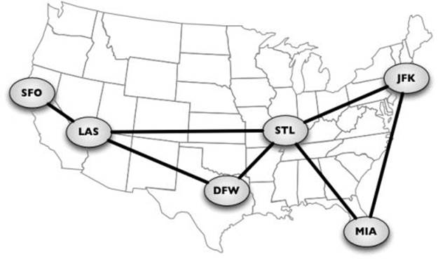
We can also use graphs to represent roads, flights, and communications, as shown in the following image:

Let's learn more about the mathematical and technical concepts of graphs.

A graph G = (V, E) is composed of:

· V: A set of vertices

· E: A set of edges connecting the vertices in V

The following diagram represents a graph:

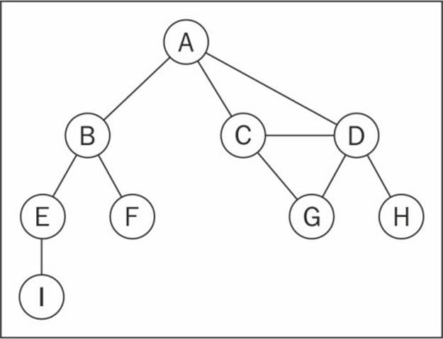
Let's cover some graph terminology before we start implementing any algorithms.

Vertices connected by an edge are called adjacent vertices. For example, A and B are adjacent, A and D are adjacent, A and C are adjacent, and A and E are not adjacent.

A degree of a vertex consists of the number of adjacent vertices. For example, A is connected to other three vertices, therefore, A has degree 3; E is connected to other two vertices, therefore, E has degree 2.

A path is a sequence of consecutive vertices v1, v2, …, vk, where vi and vi+1 are adjacent. Using the graph from the previous diagram as an example, we have paths A B E I and A C D G, among others.

A simple path does not contain repeated vertices. As an example, we have the path A D G. A cycle is a simple path, except for the last vertex, which is the same as the first vertex: A D C A (back to A).

A graph is acyclic if it does not have cycles. A graph is connected if there is a path between every pair of vertices.

Directed and undirected graphs

Graphs can be undirected (where edges do not have a direction) or directed (digraph), where edges have a direction, as demonstrated here:

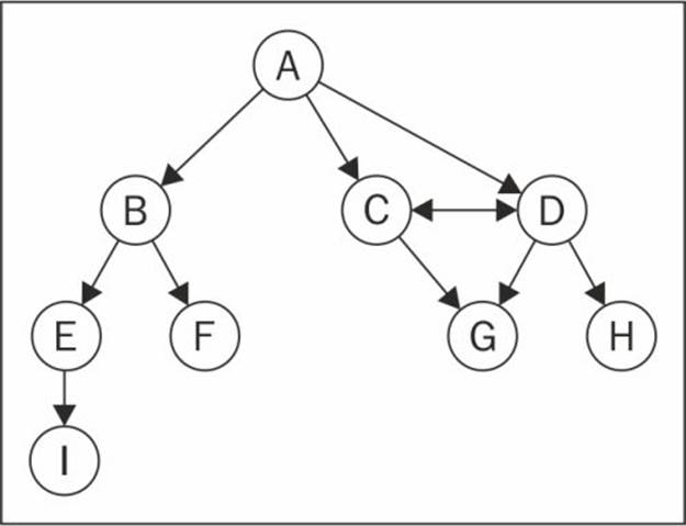
A graph is strongly connected if there is a path in both directions between every pair of vertices. For example, C and D are strongly connected while A and B are not strongly connected.

Graphs can also be unweighted (as we have seen so far) or weighted, where the edges have weights, as shown in the following diagram:

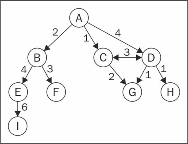
We can solve many problems in the Computer Science world using graphs, such as searching a graph for a specific vertex or searching for a specific edge, finding a path in the graph (from one vertex to another), finding the shortest path between two vertices, and cycle detection.

Representing a graph

There are a few ways we can represent graphs when it comes to data structures. There is no correct way of representing a graph among the existing possibilities. It depends on the type of problem you need to resolve and the type of graph as well.

The adjacency matrix

The most common implementation is the adjacency matrix. Each node is associated with an integer, which is the array index. We represent the connectivity between vertices using a two-dimensional array, as array[i][j] === 1 if there is an edge from the node with index i to the node with index j; or as array[i][j] === 0 otherwise, as demonstrated by the following diagram:

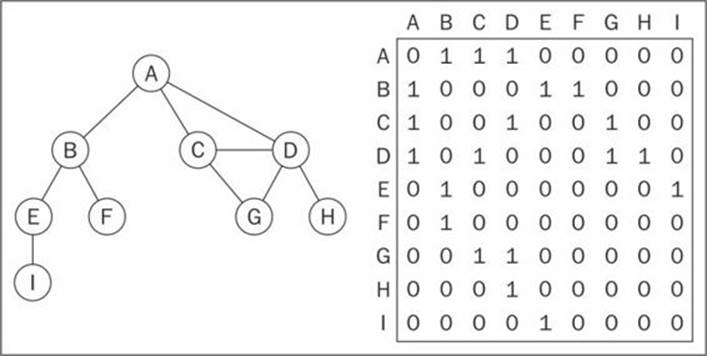
Graphs that are not strongly connected (sparse graphs) will be represented by a matrix with many zero entries in the adjacency matrix. This means we will waste space in the computer memory to represent edges that do not exist; for example, if we need to find the adjacent vertices of a given vertex, we will have to iterate through the whole row even if this vertex has only one adjacent vertex. Another reason this might not be a good representation is because the number of vertices in the graph may change and a two-dimensional array is inflexible.

The adjacency list

We can use a dynamic data structure to represent graphs as well, called an adjacency list. This consists of a list of adjacent vertices for every vertex of the graph. There are a few different ways we can represent this data structure. To represent the list of adjacent vertices, we can use a list (array), a linked list, or even a hash map or dictionary. The following diagram exemplifies the adjacency list data structure:

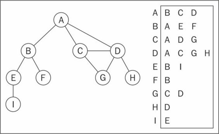
Both representations are very useful and have different properties (for example, finding out whether vertices v and w are adjacent is faster using adjacent matrix), although adjacency lists are probably better for most problems. We are going to use the adjacency list representation for the examples in this book.

The incidence matrix

We can also represent a graph using an incidence matrix. In an incidence matrix, each row of the matrix represents a vertex and each column represents an edge. We represent the connectivity between the two objects using a two-dimensional array, as array[v][e] === 1 if the vertex v is incident upon edge e; or as array[v][e] === 0 otherwise, as demonstrated in the following diagram:

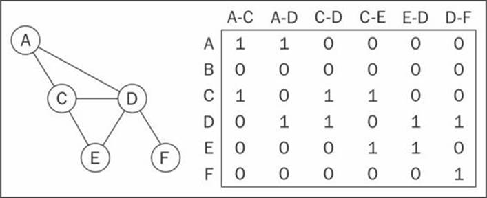
An incidence matrix is usually used to save space and memory when we have more edges than vertices.

Creating the Graph class

As usual, we are going to declare the skeleton of our class:

function Graph() {

var vertices = []; //{1}

var adjList = new Dictionary(); //{2}

}

We are going to use an array to store the names of all the vertices of the graph (line {1}) and we are going to use a dictionary (implemented in Chapter 7, Dictionaries and Hashes) to store the adjacent list (line {2}). The dictionary will use the name of the vertex as key and the list of adjacent vertices as a value. Both the vertices array and the adjList dictionary are private attributes of our Graph class.

Next, we are going to implement two methods: one to add a new vertex to the graph (because when we instantiate the graph, it will create an empty one) and another method to add edges between the vertices. Let's implement the addVertex method first:

this.addVertex = function(v){

vertices.push(v); //{3}

adjList.set(v, []); //{4}

};

This method receives a vertex v as parameter. We are going to add this vertex to the list of vertices (line {3}), and we are also going to initialize the adjacent list with an empty array by setting the dictionary value of the vertex v key with an empty array (line {4}).

Now, let's implement the addEdge method:

this.addEdge = function(v, w){

adjList.get(v).push(w); //{5}

adjList.get(w).push(v); //{6}

};

This method receives two vertices as parameters. First, we are going to add an edge from vertex v to vertex w (line {5}) by adding w to the adjacent list of v. If you want to implement a directed graph, line {5} is enough. As we are going to work with undirected graphs in most examples in this chapter, we also need to add the edge from w to v (line {6}).

Note that we are only adding new elements to the array, since we have already initialized it in line {4}.

Let's test this code:

var graph = new Graph();

var myVertices = ['A','B','C','D','E','F','G','H','I']; //{7}

for (var i=0; i<myVertices.length; i++){ //{8}

graph.addVertex(myVertices[i]);

}

graph.addEdge('A', 'B'); //{9}

graph.addEdge('A', 'C');

graph.addEdge('A', 'D');

graph.addEdge('C', 'D');

graph.addEdge('C', 'G');

graph.addEdge('D', 'G');

graph.addEdge('D', 'H');

graph.addEdge('B', 'E');

graph.addEdge('B', 'F');

graph.addEdge('E', 'I');

To make our lives easier, let's create an array with all the vertices we want to add to our graph (line {7}). Then, we only need to iterate through the vertices array and add the values one by one to our graph (line {8}). Finally, we add the desired edges (line {9}). This code will create the graph we used in the diagrams presented so far in this chapter.

To make our lives even easier, let's also implement the toString method for this Graph class, so that we can output the graph on the console:

this.toString = function(){

var s = '';

for (var i=0; i<vertices.length; i++){ //{10}

s += vertices[i] + ' -> ';

var neighbors = adjList.get(vertices[i]); //{11}

for (var j=0; j<neighbors.length; j++){ //{12}

s += neighbors[j] + ' ';

}

s += '\n'; //{13}

}

return s;

};

We are going to build a string with the adjacent list representation. First, we are going to iterate the list of vertices array (line {10}) and add the name of the vertex to our string. Then, we are going to get the adjacent list for this vertex (line {11}) and we are also going to iterate it (line {12}) to get the name of the adjacent vertex and add it to our string. After we have iterated the adjacent list, we are going to add a new line to our string (line {13}), so we can see a pretty output on the console. Let's try this code:

console.log(graph.toString());

This will be the output:

A -> B C D

B -> A E F

C -> A D G

D -> A C G H

E -> B I

F -> B

G -> C D

H -> D

I -> E

A pretty adjacent list! From this output, we know that vertex A has the following adjacent vertices: B, C, and D.

Graph traversals

Similar to the tree data structure, we can also visit all the nodes of a graph. There are two algorithms that can be used to traverse a graph called breadth-first search (BFS) and depth-first search (DFS). Traversing a graph can be used to find a specific vertex or to find a path between two vertices, check whether the graph is connected, check whether it contains cycles, and so on.

Before we implement the algorithms, let's try to better understand the idea of traversing a graph.

The idea of graph traversal algorithms is that we must track each vertex when we first visit it and keep track of which vertices have not yet been completely explored. For both traversal graph algorithms, we need to specify which is going to be the first vertex to be visited.

To completely explore a vertex, we need to look at each edge of this vertex. For each edge connected to a vertex that has not been visited yet, we mark it as discovered and add it to the list of vertices to be visited.

In order to have efficient algorithms, we must visit each vertex twice, at the most, when each of its endpoints are explored. Every edge and vertex in the connected graph will be visited.

The BFS and DFS algorithms are basically the same, with only one difference, which is the data structure used to store the list of vertices to be visited:

When marking the vertices that we have already visited, we use three colors to reflect their status:

· White: This represents that the vertex has not been visited

· Grey: This represents that the vertex has been visited but not explored

· Black: This represents that the vertex has been completely explored

This is why we must visit each vertex twice, at the most, as mentioned earlier.

Breadth-first search (BFS)

The BFS algorithm will start traversing the graph from the first specified vertex and will visit all its neighbors (adjacent vertices) first, as it is visiting each layer of the graph at a time. In other words, it visits the vertices first widely and then deeply, as demonstrated by the following diagram:

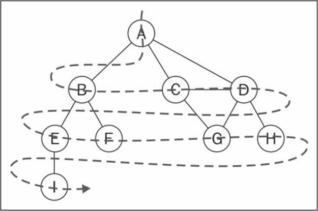
These are the steps followed by the BFS algorithm starting at vertex v:

1. Create a queue Q.

2. Mark v as discovered (grey) and enqueue v into Q.

3. While Q is not empty, perform the following steps:

1. Dequeue u from Q.

2. Mark u as discovered (grey).

3. Enqueue all unvisited (white) neighbors w of u.

4. Mark u as explored (black).

Let's implement the BFS algorithm:

var initializeColor = function(){

var color = [];

for (var i=0; i<vertices.length; i++){

color[vertices[i]] = 'white'; //{1}

}

return color;

};

this.bfs = function(v, callback){

var color = initializeColor(), //{2}

queue = new Queue(); //{3}

queue.enqueue(v); //{4}

while (!queue.isEmpty()){ //{5}

var u = queue.dequeue(), //{6}

neighbors = adjList.get(u); //{7}

color[u] = 'grey'; //{8}

for (var i=0; i<neighbors.length; i++){ //{9}

var w = neighbors[i]; //{10}

if (color[w] === 'white'){ //{11}

color[w] = 'grey'; //{12}

queue.enqueue(w); //{13}

}

}

color[u] = 'black'; //{14}

if (callback) { //{15}

callback(u);

}

}

};

For both BFS and DFS, we will need to mark the vertices visited. To do so, we will use a helper array called color. As and when we start executing the BFS or DFS algorithms, all vertices have the color white (line {1}), so we can create a helper function called initializeColor, which will do this for us for both the algorithms we are implementing.

Let's dive into the BFS method implementation. The first thing we will do is use the initializeColor function to initialize the color array with the color white (line {2}). We also need to declare and create a Queue instance (line {3}) that will store the vertices that need to be visited and explored.

Following the steps we explained at the beginning of this chapter, the bfs method receives a vertex that will be used as the point of origin for our algorithm. As we need a starting point, we will enqueue this vertex into the queue (line {4}).

If the queue is not empty (line {5}), we will remove a vertex from the queue by dequeuing it (line {6}) and we will get its adjacency list that contains all its neighbors (line {7}). We will also mark this vertex as grey, meaning we discovered it (but have not finished exploring it yet).

For each neighbor of u (line {9}), we will obtain its value (the name of the vertex—line {10}), and if it has not been visited yet (color set to white—line {11}), we will mark that we have discovered it (color is set to grey—line {12}), and will add this vertex to the queue (line {13}), so it can be finished exploring when we dequeue it from the queue.

When we finish exploring the vertex and its adjacent vertices, we mark is as explored (color is set to black—line {14}).

The bfs method we are implementing also receives a callback (we used a similar approach in Chapter 8, Trees, for tree traversals). This parameter is optional, and if we pass any callback function (line {15}), we will use it.

Let's test this algorithm by executing the following code:

function printNode(value){ //{16}

console.log('Visited vertex: ' + value); //{17}

}

graph.bfs(myVertices[0], printNode); //{18}

First, we declared a callback function (line {16}) that will simply output in the browser's console the name (line {17}) of the vertex that was completely explored by the algorithm. Then, we will call the bfs method, passing the first vertex (A—from the myVertices array that we declared at the beginning of this chapter) and the callback function. When we execute this code, the algorithm will output the following result in the browser's console:

Visited vertex: A

Visited vertex: B

Visited vertex: C

Visited vertex: D

Visited vertex: E

Visited vertex: F

Visited vertex: G

Visited vertex: H

Visited vertex: I

As you can see, the order of the vertices visited is the same as shown by the diagram at the beginning of this section.

Finding the shortest paths using BFS

So far, we have only demonstrated how the BFS algorithm works. We can use it for more things than just outputting the order of vertices visited. For example, how would we solve the following problem?

Given a graph G and the source vertex v, find the distance (in number of edges) from v to each vertex u Î G along the shortest path between v and u.

Given a vertex v, the BFS algorithm visits all vertices with distance 1, and then distance 2, and so on. So, we can use the BFS algorithm to solve this problem. We can modify the bfs method to return some information for us:

· The distances d[u] from v to u

· The predecessors pred[u], which is used to derive a shortest path from v to every other vertex u

Let' see the implementation of an improved BFS method:

this.BFS = function(v){

var color = initializeColor(),

queue = new Queue(),

d = [], //{1}

pred = []; //{2}

queue.enqueue(v);

for (var i=0; i<vertices.length; i++){ //{3}

d[vertices[i]] = 0; //{4}

pred[vertices[i]] = null; //{5}

}

while (!queue.isEmpty()){

var u = queue.dequeue(),

neighbors = adjList.get(u);

color[u] = 'grey';

for (i=0; i<neighbors.length; i++){

var w = neighbors[i];

if (color[w] === 'white'){

color[w] = 'grey';

d[w] = d[u] + 1; //{6}

pred[w] = u; //{7}

queue.enqueue(w);

}

}

color[u] = 'black';

}

return { //{8}

distances: d,

predecessors: pred

};

};

What has changed in this version of the BFS method?

Note

The source code of this chapter contains two bfs methods: bfs (the first one we implemented) and BFS (the improved one).

We also need to declare the d array (line {1}), which represents the distances and the pred array (line {2}), which represents the predecessors. The next step would be initializing the d array with 0 (zero—line {4}) and the pred array with null (line {5}) for every vertex of the graph (line {3}).

When we discover the neighbor w of a vertex u, we set the predecessor value of w as u (line {7}) and we also increment the distance (line {6}) between v and w by adding 1 and the distance of u (as u is a predecessor of w, we have the value of d[u] already).

At the end of the method, we can return an object with d and pred (line {8}).

Now, we can execute the BFS method again and store its return value in a variable:

var shortestPathA = graph.BFS(myVertices[0]);

console.log(shortestPathA);

As we executed the BFS method for the vertex A, this will be the output on the console:

distances: [A: 0, B: 1, C: 1, D: 1, E: 2, F: 2, G: 2, H: 2 , I: 3],

predecessors: [A: null, B: "A", C: "A", D: "A", E: "B", F: "B", G: "C", H: "D", I: "E"]

This means that vertex A has distance of 1 edge from vertices B, C, and D; a distance of 2 edges from vertices E, F, G, and H; and a distance of 3 edges from vertex I.

With the predecessors array, we can build the path from vertex A to the other vertices by using the following code:

var fromVertex = myVertices[0]; //{9}

for (var i=1; i<myVertices.length; i++){ //{10}

var toVertex = myVertices[i], //{11}

path = new Stack(); //{12}

for (var v=toVertex; v!== fromVertex;

v=shortestPathA.predecessors[v]) { //{13}

path.push(v); //{14}

}

path.push(fromVertex); //{15}

var s = path.pop(); //{16}

while (!path.isEmpty()){ //{17}

s += ' - ' + path.pop(); //{18}

}

console.log(s); //{19}

}

We will use vertex A as the source vertex (line {9}). For every other vertex (except vertex A—line {10}), we will calculate the path from vertex A to it. To do so, we will get the value of the toVertex method from the vertices array (line {11}), and we will create a stack to store the path values (line {12}).

Next, we will follow the path from toVertex to fromVertex (line {13}). The v variable will receive the value of its predecessor and we will be able to take the same path backwards. We will add the v variable to the stack (line {14}). Finally, we will add the origin vertex to the stack as well (line {15}) to have the complete path.

After this, we will create an s string and we will assign the origin vertex to it (this will be the last vertex added to the stack, so it is the first item to be popped out—line {16}). While the stack is not empty (line {17}), we will remove an item from the stack and will concatenate it to the existing value of the s string (line {18}). Finally (line {19}), we simply output the path on the browser's console.

After executing the previous code, we will get the following output:

A - B

A - C

A - D

A - B - E

A - B - F

A - C - G

A - D - H

A - B - E - I

Here, we have the shortest path (in number of edges) from A to the other vertices of the graph.

Further studies on the shortest paths algorithms

The graph we used in this example is not a weighted graph. If we want to calculate the shortest path in weighted graphs (for example, what the shortest path is between city A and city B—an algorithm used in GPS and Google Maps), BFS is not the indicated algorithm.

There is Dijkstra's algorithm, which solves the single-source shortest path problem for example. The Bellman–Ford algorithm solves the single-source problem if edge weights are negative. The A* search algorithm provides the shortest path for a single pair of vertices using heuristics to try to speed up the search. The Floyd–Warshall algorithm provides the shortest path for all pairs of vertices.

As mentioned on the first page of this chapter, the subject of graphs is an extensive topic, and we have many solutions for the shortest path problem and its variations. But before we start studying these other solutions, you need to learn the basic concepts of graphs, which we covered in this chapter. These other solutions will not be covered in the book, but you can have an adventure of your own exploring the amazing graph world.

Depth-first search (DFS)

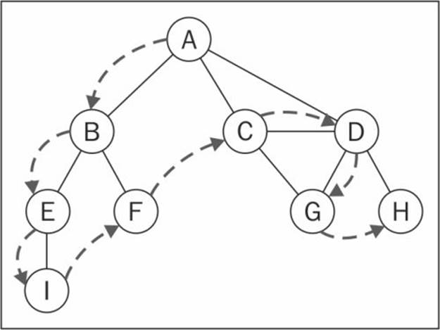
The DFS algorithm will start traversing the graph from the first specified vertex and will follow a path until the last vertex of this path is visited, and then will backtrack and then follow the next path. In another words, it visits the vertices first deeply and then widely, as demonstrated in the following diagram:

The DFS algorithm does not need a source vertex. In the DFS algorithm, for each unvisited vertex v in graph G, visit the vertex v.

To visit vertex v, do the following:

1. Mark v as discovered (grey).

2. For all unvisited (white) neighbors w of v:

1. Visit vertex w.

3. Mark v as explored (black).

As you can see, the DFS steps are recursive, meaning the DFS algorithm uses a stack to store the calls (a stack created by the recursive calls).

Let's implement the DFS algorithm:

this.dfs = function(callback){

var color = initializeColor(); //{1}

for (var i=0; i<vertices.length; i++){ //{2}

if (color[vertices[i]] === 'white'){ //{3}

dfsVisit(vertices[i], color, callback); //{4}

}

}

};

var dfsVisit = function(u, color, callback){

color[u] = 'grey'; //{5}

if (callback) { //{6}

callback(u);

}

var neighbors = adjList.get(u); //{7}

for (var i=0; i<neighbors.length; i++){ //{8}

var w = neighbors[i]; //{9}

if (color[w] === 'white'){ //{10}

dfsVisit(w, color, callback); //{11}

}

}

color[u] = 'black'; //{12}

};

The first thing we need to do is create and initialize the color array (line {1}) with the value white for each vertex of the graph. We did the same thing for the BFS algorithm. Then, for each non-visited vertex (lines {2} and {3}) of the Graph instance, we will call the recursive private functiondfsVisit, passing the vertex, the color array, and the callback function (line {4}).

Whenever we visit the u vertex, we mark it as discovered (grey—line {5}). If there is a callback function (line {6}), we will execute it to output the vertex visited. Then, the next step is getting the list of neighbors of vertex u (line {7}). For each unvisited (color white—lines {10} and {8}) neighbor w (line {9}) of u, we will call the dfsVisit function, passing w and the other parameters (line {11}—add the vertex w to the stack so it can be visited next). At the end, after the vertex and its adjacent vertices were visited deeply, we backtrack, meaning the vertex is completely explored, and is marked black (line {12}).

Let's test the dfs method by executing the following code:

graph.dfs(printNode);

This will be its output:

Visited vertex: A

Visited vertex: B

Visited vertex: E

Visited vertex: I

Visited vertex: F

Visited vertex: C

Visited vertex: D

Visited vertex: G

Visited vertex: H

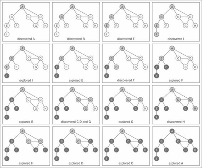
The order is the same as demonstrated by the diagram at the beginning of this section. The following diagram demonstrates the step-by-step process of the algorithm:

In this graph that we used as an example, line {4} will be executed only once, because all the other vertices have a path to the first one that called the dfsVisit function (vertex A). If vertex B is the first one to call the function, then line {4} would be executed again for another vertex (for example, vertex A).

Exploring the DFS algorithm

So far, we have only demonstrated how the DFS algorithm works. We can use it for more functions than just outputting the order of vertices visited.

Given a graph G, the DFS algorithm traverses all vertices of G and constructs a forest (a collection of rooted trees) together with a set of source vertices (roots), and outputs two arrays: discovery time and finish explorer time. We can modify the dfs method to return some information for us:

· The discovery time d[u] of u

· The finish time f[u] when u is marked black

· The predecessors p[u] of u

Let's see the implementation of the improved BFS method:

var time = 0; //{1}

this.DFS = function(){

var color = initializeColor(), //{2}

d = [],

f = [],

p = [];

time = 0;

for (var i=0; i<vertices.length; i++){ //{3}

f[vertices[i]] = 0;

d[vertices[i]] = 0;

p[vertices[i]] = null;

}

for (i=0; i<vertices.length; i++){

if (color[vertices[i]] === 'white'){

DFSVisit(vertices[i], color, d, f, p);

}

}

return { //{4}

discovery: d,

finished: f,

predecessors: p

};

};

var DFSVisit = function(u, color, d, f, p){

console.log('discovered ' + u);

color[u] = 'grey';

d[u] = ++time; //{5}

var neighbors = adjList.get(u);

for (var i=0; i<neighbors.length; i++){

var w = neighbors[i];

if (color[w] === 'white'){

p[w] = u; //{6}

DFSVisit(w,color, d, f, p);

}

}

color[u] = 'black';

f[u] = ++time; //{7}

console.log('explored ' + u);

};

As we want to track the time of discovery and time when we finished exploring, we need to declare a variable to do it (line {1}). We cannot pass time as a parameter because variables that are not objects cannot be passed as a reference to other JavaScript methods (passing a variable as a reference means that if this variable is modified inside the other method, the new values will also be reflected in the original variable). Next, we will declare the d, f, and p arrays too (line {2}). We also need to initialize these arrays for each vertex of the graph (line {3}). At the end of the method, we will return these values (line {4}) so we can work with them later.

When a vertex is first discovered, we track its discovery time (line {5}). When it is discovered as an edge from u, we also keep track of its predecessor (line {6}). At the end, when the vertex is completely explored, we track its finish time (line {7}).

What is the idea behind the DFS algorithm? The edges are explored out of the most recently discovered vertex u. Only edges to non-visited vertices are explored. When all edges of u have been explored, the algorithm backtracks to explore other edges where the vertex u was discovered. The process continues until we have discovered all the vertices that are reachable from the original source vertex. If any undiscovered vertices remain, then we repeat the process for a new source vertex. We repeat the algorithm until all vertices from the graph are explored.

There are two things we need to check for the improved DFS algorithm:

· The time variable can only have values from one to two times the number of vertices of the graph (2|V|)

· For all vertices u, d[u] < f[u] (meaning the discovered time needs to have a lower value than the finish time—meaning all the vertices have been explored)

With these two assumptions, we have the following rule:

1 ≤ d[u] < f[u] ≤ 2|V|

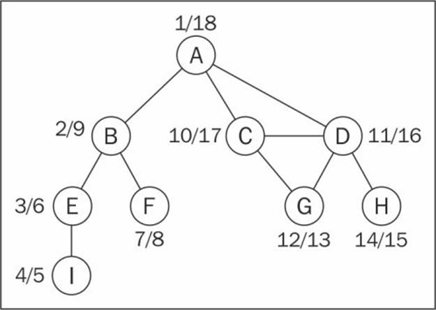
If we run the new DFS method for the same graph again, we will get the following discovery/finish time for each vertex of the graph:

But what can we do with this information? Let's see in the following section.

Topological sorting using DFS

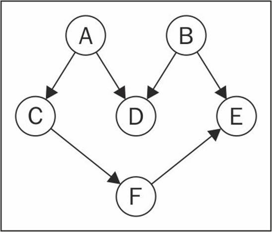
Given the following graph, suppose each vertex is a task that you need to execute:

Note

This is a directed graph, meaning there is an order that the tasks need to be executed. For example, task F cannot be executed before task A. Note that the previous graph also does not have a cycle, meaning it is an acyclic graph. So, we can say that the previous graph is a directed acyclic graph (DAG).

When we need to specify the order that some tasks or steps need to be executed in, it is called topological sorting (or topsort or even toposort). This problem is present in different scenarios of our lives. For example, when we start a Computer Science course, there is an order of disciplines we can take before taking any other discipline (you cannot take Algorithms II before taking Algorithms I). When we are working in a development project, there are some steps that need to be executed in order, for example, first we need to get the requirements from the client, then develop what was asked by the client, and then deliver the project. You cannot deliver the project and after that gather the requirements.

Topological sorting can only be applied to DAGs. So, how can we use topological sorting using DFS? Let's execute the DFS algorithm for the diagram presented at the beginning of this topic:

graph = new Graph();

myVertices = ['A','B','C','D','E','F'];

for (i=0; i<myVertices.length; i++){

graph.addVertex(myVertices[i]);

}

graph.addEdge('A', 'C');

graph.addEdge('A', 'D');

graph.addEdge('B', 'D');

graph.addEdge('B', 'E');

graph.addEdge('C', 'F');

graph.addEdge('F', 'E');

var result = graph.DFS();

This code will create the graph, apply the edges, execute the improved DFS algorithm, and store the results inside the result variable. The following diagram demonstrates the discovery and finish times of the graph after DFS is executed:

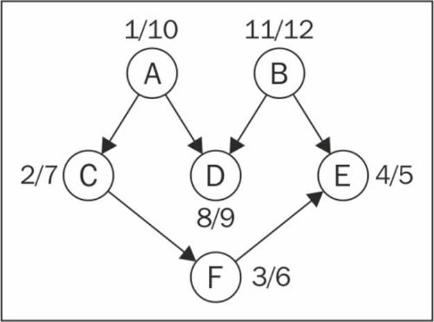
Now all we have to do is sort the finishing time array in decreased order of finishing time and we have the topological sorting for the graph:

B - A - D - C - F - E

Note that the previous toposort result is only one of the possibilities. There might be different results if we modify the algorithm a little bit, for example, the following result is one of the many other possibilities:

A - B - C - D - F - E

This could also be an acceptable result.

Summary

In this chapter, we covered the basic concepts of graphs. We learned the different ways we can represent this data structure and we implemented an algorithm to represent a graph using adjacency list. You also learned how to traverse a graph using BFS and DFS approaches. This chapter also covered two applications of BFS and DFS, which are finding the shortest path using BFS and topological sorting using DFS.

In the next chapter, you will learn the most common sorting algorithms used in Computer Science.