Wiley Linux Command Line and Shell Scripting Bible 3rd (2015)

Part I. The Linux Command Line

Chapter 8. Managing Filesystems

In This Chapter

1. Understanding filesystem basics

2. Exploring journaling and copy-on-write filesystems

3. Managing filesystems

4. Investigating the logical volume layout

5. Using the Linux Logical Volume Manager

When you're working with your Linux system, one of the decisions you'll need to make is what filesystem to use for the storage devices. Most Linux distributions kindly provide a default filesystem for you at installation time, and most beginning Linux users just use it without giving the topic another thought.

Although using the default filesystem choice isn't necessarily a bad thing, sometimes it helps to know the other options available to you. This chapter discusses the different filesystem options you have available in the Linux world and shows you how to create and manage them from the Linux command line.

Exploring Linux Filesystems

Chapter 3 discussed how Linux uses a filesystem to store files and folders on a storage device. The filesystem provides a way for Linux to bridge the gap between the ones and zeroes stored in the hard drive and the files and folders you work with in your applications.

Linux supports several types of filesystems to manage files and folders. Each filesystem implements the virtual directory structure on storage devices using slightly different features. This section walks you through the strengths and weaknesses of the more common filesystems used in the Linux environment.

Understanding the basic Linux filesystems

The original Linux system used a simple filesystem that mimicked the functionality of the Unix filesystem. This section discusses the evolution of that filesystem.

Looking at the ext Filesystem

The original filesystem introduced with the Linux operating system is called the extended filesystem (or just ext for short). It provides a basic Unix-like filesystem for Linux, using virtual directories to handle physical devices, and storing data in fixed-length blocks on the physical devices.

The ext filesystem uses a system called inodes to track information about the files stored in the virtual directory. The inode system creates a separate table on each physical device, called the inode table, to store file information. Each stored file in the virtual directory has an entry in the inode table. The extended part of the name comes from the additional data that it tracks on each file, which consists of these items:

· The filename

· The file size

· The owner of the file

· The group the file belongs to

· Access permissions for the file

· Pointers to each disk block that contains data from the file

Linux references each inode in the inode table using a unique number (called the inode number), assigned by the filesystem as data files are created. The filesystem uses the inode number to identify the file rather than having to use the full filename and path.

Looking at the ext2 Filesystem

The original ext filesystem had quite a few limitations, such as restraining files to only 2GB in size. Not too long after Linux was first introduced, the ext filesystem was upgraded to create the second extended filesystem, called ext2.

As you can guess, the ext2 filesystem is an expansion of the basic abilities of the ext filesystem, but maintains the same structure. The ext2 filesystem expands the inode table format to track additional information about each file on the system.

The ext2 inode table adds the created, modified, and last accessed time values for files to help system administrators track file access on the system. The ext2 filesystem also increases the maximum file size allowed to 2TB (then in later versions of ext2, that was increased to 32TB) to help accommodate large files commonly found in database servers.

In addition to expanding the inode table, the ext2 filesystem also changed the way in which files are stored in the data blocks. A common problem with the ext filesystem was that as a file is written to the physical device, the blocks used to store the data tend to be scattered throughout the device (called fragmentation). Fragmentation of data blocks can reduce the filesystem performance, because it takes longer to search the storage device to access all the blocks for a specific file.

The ext2 filesystem helps reduce fragmentation by allocating disk blocks in groups when you save a file. By grouping the data blocks for a file, the filesystem doesn't have to search all over the physical device for the data blocks to read the file.

The ext2 filesystem was the default filesystem used in Linux distributions for many years, but it, too, had its limitations. The inode table, although a nice feature that allows the filesystem to track additional information about files, can cause problems that can be fatal to the system. Each time the filesystem stores or updates a file, it must modify the inode table with the new information. The problem is that this isn't always a fluid action.

If something should happen to the computer system between the file being stored and the inode table being updated, the two would become out of sync. The ext2 filesystem is notorious for easily becoming corrupted due to system crashes and power outages. Even if the file data is stored just fine on the physical device, if the inode table entry isn't completed, the ext2 filesystem doesn't even know that the file existed!

It wasn't long before developers were exploring a different avenue of Linux filesystems.

Understanding journaling filesystems

Journaling filesystems provide a new level of safety to the Linux system. Instead of writing data directly to the storage device and then updating the inode table, journaling filesystems write file changes into a temporary file (called the journal) first. After data is successfully written to the storage device and the inode table, the journal entry is deleted.

If the system should crash or suffer a power outage before the data can be written to the storage device, the journaling filesystem just reads through the journal file and processes any uncommitted data left over.

Linux commonly uses three different methods of journaling, each with different levels of protection. These are shown in Table 8.1.

Table 8.1 Journaling Filesystem Methods

The data mode journaling method is by far the safest for protecting data, but it is also the slowest. All the data written to a storage device must be written twice, once to the journal and again to the actual storage device. This can cause poor performance, especially for systems that do lots of data writing.

Over the years, a few different journaling filesystems have appeared in Linux. The following sections describe the popular Linux journaling filesystems available.

Looking at the ext3 Filesystem

The ext3 filesystem was added to the Linux kernel in 2001, and up until recently was the default filesystem used by just about all Linux distributions. It uses the same inode table structure as the ext2 filesystem, but adds a journal file to each storage device to journal the data written to the storage device.

By default, the ext3 filesystem uses the ordered mode method of journaling, only writing the inode information to the journal file, but not removing it until the data blocks have been successfully written to the storage device. You can change the journaling method used in the ext3 filesystem to either data or writeback modes with a simple command line option when creating the filesystem.

Although the ext3 filesystem added basic journaling to the Linux filesystem, it still lacked a few things. For example, the ext3 filesystem doesn't provide any recovery from accidental deletion of files, no built-in data compression is available (although a patch can be installed separately that provides this feature), and the ext3 filesystem doesn't support encrypting files. For those reasons, developers in the Linux project chose to continue work on improving the ext3 filesystem.

Looking at the ext4 Filesystem

The result of expanding the ext3 filesystem was (as you probably guessed) the ext4 filesystem. The ext4 filesystem was officially supported in the Linux kernel in 2008 and is now the default filesystem used in popular Linux distributions, such as Ubuntu.

In addition to supporting compression and encryption, the ext4 filesystem also supports a feature called extents. Extents allocate space on a storage device in blocks and only store the starting block location in the inode table. This helps save space in the inode table by not having to list all the data blocks used to store data from the file.

The ext4 filesystem also incorporates block preallocation. If you want to reserve space on a storage device for a file that you know will grow in size, with the ext4 filesystem it's possible to allocate all the expected blocks for the file, not just the blocks that physically exist. The ext4 filesystem fills in the reserved data blocks with zeroes and knows not to allocate them for any other file.

Looking at the Reiser Filesystem

In 2001, Hans Reiser created the first journaling filesystem for Linux, called ReiserFS. The ReiserFS filesystem supports only writeback journaling mode, writing only the inode table data to the journal file. Because it writes only the inode table data to the journal, the ReiserFS filesystem is one of the faster Linux journaling filesystems.

Two interesting features incorporated into the ReiserFS filesystem are that you can resize an existing filesystem while it's still active and that it uses a technique called tailpacking, which stuffs data from one file into empty space in a data block from another file. The active filesystem resizing feature is great if you have to expand an already created filesystem to accommodate more data.

The ReiserFS development team began working on a new version called Reiser4 in 2004. The Reiser4 filesystem has several improvements over ResierFS, including extremely efficient handling of small files. However, most current mainstream Linux distributions don't use the Reiser4 filesystem. Yet, you may still run into a Linux system that employs it.

Looking at the Journaled Filesystem

Possibly one of the oldest journaling filesystems around, the Journaled File System (JFS) was developed by IBM in 1990 for its AIX flavor of Unix. However, it wasn't until its second version that it was ported to the Linux environment.

Note

The official IBM name of the second version of the JFS filesystem is JFS2, but most Linux systems refer to it as just JFS.

The JFS filesystem uses the ordered journaling method, storing only the inode table data in the journal, but not removing it until the actual file data is written to the storage device. This method is a compromise between the speed of the Reiser4 and the integrity of the data mode journaling method.

The JFS filesystem uses extent-based file allocation, allocating a group of blocks for each file written to the storage device. This method provides for less fragmentation on the storage device.

Outside of the IBM Linux offerings, the JFS filesystem isn't popularly used, but you may run into it in your Linux journey.

Looking at the XFS Filesystem

The XFS journaling filesystem is yet another filesystem originally created for a commercial Unix system that made its way into the Linux world. Silicon Graphics Incorporated (SGI) originally created XFS in 1994 for its commercial IRIX Unix system. It was released to the Linux environment for common use in 2002. The XFS filesystem has recently become more popular and is used as the default filesystem in mainstream Linux distributions, such as RHEL.

The XFS filesystem uses the writeback mode of journaling, which provides high performance but does introduce an amount of risk because the actual data isn't stored in the journal file. The XFS filesystem also allows online resizing of the filesystem, similar to the Reiser4 filesystem, except XFS filesystems can only be expanded and not shrunk.

Understanding the copy-on-write filesystems

With journaling, you must choose between safety and performance. Although data mode journaling provides the highest safety, performance suffers because both inode and data is journaled. With writeback mode journaling, performance is acceptable, but safety is compromised.

For filesystems, an alternative to journaling is a technique called copy-on-write (COW). COW offers both safety and performance via snapshots. For modifying data, a clone or writable-snapshot is used. Instead of writing modified data over current data, the modified data is put in a new filesystem location. Even when data modification is completed, the old data is never overwritten.

COW filesystems are gaining in popularity. Two of the most popular, Btrfs and ZFS, are briefly reviewed in the following sections.

Looking at the ZFS Filesystem

The COW filesystem ZFS was developed in 2005 by Sun Microsystems for the OpenSolaris operating system. It began being ported to Linux in 2008 and was finally available for Linux production use in 2012.

ZFS is a stable filesystem and competes well against Resier4, Btrfs, and ext4. Its biggest detractor is that ZFS does not have a GPL license. The OpenZFS project was launched in 2013, which may help to change this situation. However, it's possible that until a GPL license is obtained, ZFS will never be a default Linux filesystem.

Looking at the Btrfs Filesystem

The COW newcomer is the Btrfs filesystem, also called the B-tree filesystem. Oracle started development on Btrfs in 2007. It was based on many of Reiser4's features, but offered improvements in reliability. Additional developers eventually joined in and helped Btrfs quickly rise toward the top of the popular filesystems list. This popularity is due to stability, ease of use, as well as the ability to dynamically resize a mounted filesystem. The openSUSE Linux distribution recently established Btrfs as its default filesystem. It is also offered in other Linux distributions, such as RHEL, although not as the default filesystem.

Working with Filesystems

Linux provides a few different utilities that make it easier to work with filesystems from the command line. You can add new filesystems or change existing filesystems from the comfort of your own keyboard. This section walks you through the commands for interacting with filesystems from a command line environment.

Creating partitions

To start out, you need to create a partition on the storage device to contain the filesystem. The partition can be an entire disk or a subset of a disk that contains a portion of the virtual directory.

The fdisk utility is used to help you organize partitions on any storage device installed on the system. The fdisk command is an interactive program that allows you to enter commands to walk through the steps of partitioning a hard drive.

To start the fdisk command, you need to specify the device name of the storage device you want to partition and you need to have superuser privileges. When you don't have superuser privileges and attempt to use fdisk, you'll receive some sort of error message, like this one:

$ fdisk /dev/sdb

Unable to open /dev/sdb

$

Note

Sometimes, the hardest part of creating a new disk partition is trying to find the physical disk on your Linux system. Linux uses a standard format for assigning device names to hard drives, but you need to be familiar with the format. For older IDE drives, Linux uses /dev/hdx, where x is a letter based on the order the drive is detected (a for the first drive, b for the second, and so on). For both the newer SATA drives and SCSI drives, Linux uses /dev/sdx, where x is a letter based on the order the drive is detected (again, a for the first drive, b for the second, and so on). It's always a good idea to double-check to make sure you are referencing the correct drive before formatting the partition!

If you do have superuser privileges and the correct device name, the fdisk command allows you entrance into the utility as demonstrated here on a CentOS distribution:

$ sudo fdisk /dev/sdb

[sudo] password for Christine:

Device contains neither a valid DOS partition table,

nor Sun, SGI or OSF disklabel

Building a new DOS disklabel with disk identifier 0xd3f759b5.

Changes will remain in memory only

until you decide to write them.

After that, of course, the previous content won't be recoverable.

Warning: invalid flag 0x0000 of partition table 4 will

be corrected by w(rite)

[...]

Command (m for help):

Tip

If this is the first time you're partitioning the storage device, fdisk gives you a warning that a partition table is not on the device.

The fdisk interactive command prompt uses single letter commands to instruct fdisk what to do. Table 8.2 shows the commands available at the fdisk command prompt.

Table 8.2 The fdisk Commands

Although this list may look intimidating, usually you need just a few basic commands in day-to-day work.

For starters, you can display the details of a storage device using the p command:

Command (m for help): p

Disk /dev/sdb: 5368 MB, 5368709120 bytes

255 heads, 63 sectors/track, 652 cylinders

Units = cylinders of 16065 * 512 = 8225280 bytes

Sector size (logical/physical): 512 bytes / 512 bytes

I/O size (minimum/optimal): 512 bytes / 512 bytes

Disk identifier: 0x11747e88

Device Boot Start End Blocks Id System

Command (m for help):

The output shows that the storage device has 5368MB of space on it (5GB). The listing under the storage device details shows whether there are any existing partitions on the device. The listing in this example doesn't show any partitions, so the device is not partitioned yet.

Next, you'll want to create a new partition on the storage device. Use the n command for that:

Command (m for help): n

Command action

e extended

p primary partition (1-4)

p

Partition number (1-4): 1

First cylinder (1-652, default 1): 1

Last cylinder, +cylinders or +size{K,M,G} (1-652, default 652): +2G

Command (m for help):

Partitions can be created as either a primary partition or an extended partition. Primary partitions can be formatted with a filesystem directly, whereas extended partitions can only contain other primary partitions. The reason for extended partitions is that there can only be four partitions on a single storage device. You can extend that by creating multiple extended partitions and then creating primary partitions inside the extended partitions. This example creates a primary storage device, assigns it partition number 1, and then allocates 2GB of the storage device space to it. You can see the results using the p command again:

Command (m for help): p

Disk /dev/sdb: 5368 MB, 5368709120 bytes

255 heads, 63 sectors/track, 652 cylinders

Units = cylinders of 16065 * 512 = 8225280 bytes

Sector size (logical/physical): 512 bytes / 512 bytes

I/O size (minimum/optimal): 512 bytes / 512 bytes

Disk identifier: 0x029aa6af

Device Boot Start End Blocks Id System

/dev/sdb1 1 262 2104483+ 83 Linux

Command (m for help):

Now in the output there's a partition shown on the storage device (called /dev/sdb1). The Id entry defines how Linux treats the partition. fdisk allows you to create lots of partition types. Using the l command lists the different types available. The default is type 83, which defines a Linux filesystem. If you want to create a partition for a different filesystem (such as a Windows NTFS partition), just select a different partition type.

You can repeat the process to allocate the remaining space on the storage device to another Linux partition. After you've created the partitions you want, use the w command to save the changes to the storage device:

Command (m for help): w

The partition table has been altered!

Calling ioctl() to re-read partition table.

Syncing disks.

$

The storage device partition information was written to the partition table, and Linux was informed of the new partition via the ioctl() call. Now that you have set up a partition on the storage device, you're ready to format it with a Linux filesystem.

Tip

Some distributions and older distribution versions do not automatically inform your Linux system of a new partition after it is made. In this case, you need to use either the partprobe or hdparm command (see their man pages), or reboot your system so it reads the updated partition table

Creating a filesystem

Before you can store data on the partition, you must format it with a filesystem so Linux can use it. Each filesystem type uses its own command line program to format partitions. Table 8.3 lists the utilities used for the different filesystems discussed in this chapter.

Table 8.3 Command Line Programs to Create Filesystems

Not all filesystem utilities are installed by default. To determine whether you have a particular filesystem utility, use the type command:

$ type mkfs.ext4

mkfs.ext4 is /sbin/mkfs.ext4

$

$ type mkfs.btrfs

-bash: type: mkfs.btrfs: not found

$

The preceding example on an Ubuntu system shows that the mkfs.ext4 utility is available. However, the Btrfs utility is not. See Chapter 9 on how to install additional software and utilities on your Linux distribution.

Each filesystem utility command has lots of command line options that allow you to customize just how the filesystem is created in the partition. To see all the command line options available, use the man command to display the manual pages for the filesystem command (see Chapter 3). All the filesystem commands allow you to create a default filesystem with just the simple command with no options:

$ sudo mkfs.ext4 /dev/sdb1

[sudo] password for Christine:

mke2fs 1.41.12 (17-May-2010)

Filesystem label=

OS type: Linux

Block size=4096 (log=2)

Fragment size=4096 (log=2)

Stride=0 blocks, Stripe width=0 blocks

131648 inodes, 526120 blocks

26306 blocks (5.00%) reserved for the super user

First data block=0

Maximum filesystem blocks=541065216

17 block groups

32768 blocks per group, 32768 fragments per group

7744 inodes per group

Superblock backups stored on blocks:

32768, 98304, 163840, 229376, 294912

Writing inode tables: done

Creating journal (16384 blocks): done

Writing superblocks and filesystem accounting information: done

This filesystem will be automatically checked every 23 mounts or

180 days, whichever comes first. Use tune2fs -c or -i to override.

$

The new filesystem uses the ext4 filesystem type, which is a journaling filesystem in Linux. Notice that part of the creation process was to create the new journal.

After you create the filesystem for a partition, the next step is to mount it on a virtual directory mount point so you can store data in the new filesystem. You can mount the new filesystem anywhere in your virtual directory where you need the extra space.

$ ls /mnt

$

$ sudo mkdir /mnt/my_partition

$

$ ls -al /mnt/my_partition/

$

$ ls -dF /mnt/my_partition

/mnt/my_partition/

$

$ sudo mount -t ext4 /dev/sdb1 /mnt/my_partition

$

$ ls -al /mnt/my_partition/

total 24

drwxr-xr-x. 3 root root 4096 Jun 11 09:53 .

drwxr-xr-x. 3 root root 4096 Jun 11 09:58 ..

drwx------. 2 root root 16384 Jun 11 09:53 lost+found

$

The mkdir command (Chapter 3) creates the mount point in the virtual directory, and the mount command adds the new hard drive partition to the mount point. The -t option on the mount command indicates what filesystem type, ext4, you are mounting. Now you can save new files and folders on the new partition!

Note

This method of mounting a filesystem only temporarily mounts the filesystem. When you reboot your Linux system, the filesystem doesn't automatically mount. To force Linux to automatically mount the new filesystem at boot time, add the new filesystem to the /etc/fstab file.

Now that the filesystem is mounted within the virtual directory system, it can start to be used on a regular basis. Unfortunately, with regular use comes the potential for serious problems, such as filesystem corruption. The next section looks at how to deal with these issues.

Checking and repairing a filesystem

Even with modern filesystems, things can go wrong if power is unexpectedly lost, or if a wayward application locks up the system while file access is in progress. Fortunately, some command line tools are available to help you make an attempt to restore the filesystem back to order.

Each filesystem has its own recovery command for interacting with the filesystem. That has the potential of getting ugly, because more and more filesystems are available in the Linux environment, making for lots of individual commands you have to know. Fortunately, a common front-end program available can determine the filesystem on the storage device and use the appropriate filesystem recovery command based on the filesystem being recovered.

The fsck command is used to check and repair most Linux filesystem types, including ones discussed earlier in this chapter — ext, ext2, ext3, ext4, Reiser4, JFS, and XFS. The format of the command is:

fsck options filesystem

You can list multiple filesystem entries on the command line to check. Filesystems can be referenced using either the device name, the mount point in the virtual directory, or a special Linux UUID value assigned to the filesystem.

Tip

Although journaling filesystems users do need the fsck command, it is arguable as to whether COW filesystems users do. In fact, the ZFS filesystem does not even have an interface to the fsck utility

The fsck command uses the /etc/fstab file to automatically determine the filesystem on a storage device that's normally mounted on the system. If the storage device isn't normally mounted (such as if you just created a filesystem on a new storage device), you need to use the -t command line option to specify the filesystem type. Table 8.4 lists the other command line options available.

Table 8.4 The fsck Command Line Options

You may notice that some of the command line options are redundant. That's part of the problem of trying to implement a common front-end for multiple commands. Some of the individual filesystem repair commands have additional options that can be used. If you need to do more advanced error checking, you'll need to check the man pages for the individual filesystem repair tool to see if there are extended options specific to that filesystem.

Tip

You can run the fsck command on unmounted filesystems only. For most filesystems, you can just unmount the filesystem to check it and then remount it when you're finished. However, because the root filesystem contains all the core Linux commands and log files, you can't unmount it on a running system.

This is a time where having a Linux LiveCD comes in handy! Just boot your system with the LiveCD, and then run the fsck command on the root filesystem!

This chapter has showed how to handle filesystems contained in physical storage devices. Linux also provides a couple of different ways to create logical storage devices for filesystems. The next section examines how you can use a logical storage device for your filesystems.

Managing Logical Volumes

If you create your filesystems using standard partitions on hard drives, trying to add additional space to an existing filesystem can be somewhat of a painful experience. You can only expand a partition to the extent of the available space on the same physical hard drive. If no more space is available on that hard drive, you're stuck having to get a larger hard drive and manually moving the existing filesystem to the new drive.

What would come in handy is a way to dynamically add more space to an existing filesystem by just adding a partition from another hard drive to the existing filesystem. The Linux Logical Volume Manager (LVM) software package allows you to do just that. It provides an easy way for you to manipulate disk space on a Linux system without having to rebuild entire filesystems.

Exploring logical volume management layout

The core of logical volume management is how it handles the physical hard drive partitions installed on the system. In the logical volume management world, hard drives are called physical volumes (PV). Each PV maps to a specific physical partition created on a hard drive.

Multiple PV elements are pooled together to create a volume group (VG). The logical volume management system treats the VG like a physical hard drive, but in reality the VG may consist of multiple physical partitions spread across multiple hard drives. The VG provides a platform to create the logical partitions, which actually contain the filesystem.

The final layer in the structure is the logical volume (LV). The LV creates the partition environment for Linux to create a filesystem, acting similar to a physical hard disk partition as far as Linux is concerned. The Linux system treats the LV just like a physical partition. You can format the LV using any one of the standard Linux filesystems and then add it to the Linux virtual directory at a mount point.

Figure 8.1 shows the basic layout of a typical Linux logical volume management environment.

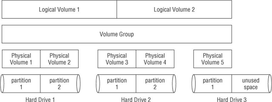
Figure 8.1 The logical volume management environment

The volume group, shown in Figure 8.1, spans across three separate physical hard drives, which contain five separate physical partitions. Inside the volume group are two separate logical volumes. The Linux system treats each logical volume just like a physical partition. Each logical volume can be formatted as an ext4 filesystem and then mounted to a specific location in the virtual directory.

Notice in Figure 8.1 that the third physical hard drive has an unused partition. Using logical volume management, you can easily assign this unused partition to the existing volume group at a later time, and then either use it to create a new logical volume or add it to expand one of the existing logical volumes when you need more space.

Likewise, if you add a new hard drive to the system, the local volume management system allows you to add it to the existing volume group, and then create more space for one of the existing logical volumes, or start a new logical volume to be mounted. That's a much better way of handling expanding filesystems!

Using the LVM in Linux

The Linux LVM was developed by Heinz Mauelshagen and released to the Linux community in 1998. It allows you to manage a complete logical volume management environment in Linux using simple command line commands.

Two versions of Linux LVM are available:

· LVM1: The original LVM package released in 1998 and available in only the 2.4 Linux kernels. It provides only basic logical volume management features.

· LVM2: An updated version of the LVM, available in the 2.6 Linux kernels. It provides additional features over the standard LVM1 features.

Most modern Linux distributions using the 2.6 kernel version or above provide support for LVM2. Besides the standard logical volume management features, LVM2 provides a few other nice things for you to use in your Linux system.

Taking a Snapshot

The original Linux LVM allows you to copy an existing logical volume to another device while the logical volume is active. This feature is called a snapshot. Snapshots are great for backing up important data that can't be locked due to high availability requirements. Traditional backup methods usually lock files as they're being copied to the backup media. The snapshot allows you to continue running mission critical web or database servers while performing the copy. Unfortunately, LVM1 allows you to create only a read-only snapshot. After you create the snapshot, you can't write to it.

LVM2 allows you to create a read-write snapshot of an active logical volume. With the read-write copy, you can remove the original logical volume and mount the snapshot as a replacement. This feature is great for fast fail-overs or for experimenting with applications that modify data that may need to be restored if something fails.

Striping

Another interesting feature that LVM2 provides is striping. With striping, a logical volume is created across multiple physical hard drives. When the Linux LVM writes a file to the logical volume, the data blocks in the file are spread across the multiple hard drives. Each successive block of data is written to the next hard drive.

Striping helps improve disk performance, because Linux can write the multiple data blocks for a file to the multiple hard drives simultaneously, rather than having to wait for a single hard drive to move the read/write head to different locations. This improvement also applies to reading sequentially accessed files, because the LVM can read data from the multiple hard drives simultaneously.

Note

LVM striping is not the same as RAID striping. LVM striping doesn't provide a parity entry, which creates the fault-tolerant environment. In fact, LVM striping may increase the chance of a file being lost due to a hard drive failure. A single disk failure can result in multiple logical volumes being inaccessible.

Mirroring

Just because you install a filesystem using LVM doesn't mean that things can't still go wrong in the filesystem. Just as in a physical partition, LVM logical volumes are susceptible to power outages and disk crashes. After a filesystem becomes corrupt, there's always a possibility that you won't be able to recover it.

The LVM snapshot process provides some comfort knowing that you can create a backup copy of a logical volume at any time, but for some environments that may not be enough. Systems that have lots of data changes, such as database servers, may store hundreds or thousands of records since the last snapshot.

A solution to this problem is the LVM mirror. A mirror is a complete copy of a logical volume that's updated in real time. When you create the mirror logical volume, LVM synchronizes the original logical volume to the mirror copy. Depending on the size of the original logical volume, this may take some time to complete.

After the original synchronization is complete, LVM performs two writes for each write process in the filesystem — one to the main logical volume and one to the mirrored copy. As you can guess, this process does slow down write performance on the system. However, if the original logical volume should become corrupt for some reason, you have a complete up-to-date copy at your fingertips!

Using the Linux LVM

Now that you've seen what the Linux LVM can do, this section discusses how to implement it to help organize the disk space on your system. The Linux LVM package only provides command line programs for creating and managing all the components in the logical volume management system. Some Linux distributions include graphical front-ends to the command line commands, but for complete control of your LVM environment, it's best to get comfortable working directly with the commands.

Defining Physical Volumes

The first step in the process is to convert the physical partitions on the hard drive into physical volume extents used by the Linux LVM. Our friend the fdisk command helps us here. After creating the basic Linux partition, you need to change the partition type using the t command:

[...]

Command (m for help): t

Selected partition 1

Hex code (type L to list codes): 8e

Changed system type of partition 1 to 8e (Linux LVM)

Command (m for help): p

Disk /dev/sdb: 5368 MB, 5368709120 bytes

255 heads, 63 sectors/track, 652 cylinders

Units = cylinders of 16065 * 512 = 8225280 bytes

Sector size (logical/physical): 512 bytes / 512 bytes

I/O size (minimum/optimal): 512 bytes / 512 bytes

Disk identifier: 0xa8661341

Device Boot Start End Blocks Id System

/dev/sdb1 1 262 2104483+ 8e Linux LVM

Command (m for help): w

The partition table has been altered!

Calling ioctl() to re-read partition table.

Syncing disks.

$

The 8e partition type denotes that the partition will be used as part of a Linux LVM system and not as a direct filesystem, as you saw with the 83 partition type earlier.

Note

If the pvcreate command in the next step does not work for you, it's most likely due to the LVM2 package not being installed by default. To install the package, use the package name lvm2 and see Chapter 9 for how to install software packages.

The next step is to use the partition to create the actual physical volume. That's done using the pvcreate command. The pvcreate command defines the physical partition to use for the PV. It simply tags the partition as a physical volume in the Linux LVM system:

$ sudo pvcreate /dev/sdb1

dev_is_mpath: failed to get device for 8:17

Physical volume "/dev/sdb1" successfully created

$

Note

Don't let the daunting message dev_is_mpath: failed to get device for 8:17 or similar messages frighten you. As long as you receive the successfully created message, all is well. The pvcreate command checks to see whether the partition is a multi-path (mpath) device. If it is not, it issues the daunting message.

You can use the pvdisplay command to display a list of physical volumes you've created if you'd like to see your progress along the way:

$ sudo pvdisplay /dev/sdb1

"/dev/sdb1" is a new physical volume of "2.01 GiB"

--- NEW Physical volume ---

PV Name /dev/sdb1

VG Name

PV Size 2.01 GiB

Allocatable NO

PE Size 0

Total PE 0

Free PE 0

Allocated PE 0

PV UUID 0FIuq2-LBod-IOWt-8VeN-tglm-Q2ik-rGU2w7

$

The pvdisplay command shows that /dev/sdb1 is now tagged as a PV. Notice, however, that in the output, the VG Name is blank. The PV does not yet belong to a volume group.

Creating Volume Groups

The next step in the process is to create one or more volume groups from the physical volumes. There are no set rules for how many volume groups you need to create for your system — you can add all the available physical volumes to a single volume group, or you can create multiple volume groups by combining different physical volumes.

To create the volume group from the command line, you need to use the vgcreate command. The vgcreate command requires a few command line parameters to define the volume group name, as well as the name of the physical volumes you're using to create the volume group:

$ sudo vgcreate Vol1 /dev/sdb1

Volume group "Vol1" successfully created

$

That's not all too exciting for output! If you'd like to see some details about the newly created volume group, use the vgdisplay command:

$ sudo vgdisplay Vol1

--- Volume group ---

VG Name Vol1

System ID

Format lvm2

Metadata Areas 1

Metadata Sequence No 1

VG Access read/write

VG Status resizable

MAX LV 0

Cur LV 0

Open LV 0

Max PV 0

Cur PV 1

Act PV 1

VG Size 2.00 GiB

PE Size 4.00 MiB

Total PE 513

Alloc PE / Size 0 / 0

Free PE / Size 513 / 2.00 GiB

VG UUID oe4I7e-5RA9-G9ti-ANoI-QKLz-qkX4-58Wj6e

$

This example creates a volume group named Vol1, using the physical volume created on the /dev/sdb1 partition.

Now that you have one or more volume groups created, you're ready to create the logical volume.

Creating Logical Volumes

The logical volume is what the Linux system uses to emulate a physical partition, and it holds the filesystem. The Linux system handles the logical volumes just like a physical partition, allowing you to define filesystems in the logical volume and then mount the filesystem into the virtual directory.

To create the logical volume, use the lvcreate command. Although you can usually get away without using command line options in the other Linux LVM commands, the lvcreate command requires at least some options to be entered. Table 8.5 shows the available command line options.

Table 8.5 The lvcreate Options

Although the command line options may look intimidating, for most situations, you can get by with a minimal amount of options:

$ sudo lvcreate -l 100%FREE -n lvtest Vol1

Logical volume "lvtest" created

$

If you want to see the details of what you created, use the lvdisplay command:

$ sudo lvdisplay Vol1

--- Logical volume ---

LV Path /dev/Vol1/lvtest

LV Name lvtest

VG Name Vol1

LV UUID 4W2369-pLXy-jWmb-lIFN-SMNX-xZnN-3KN208

LV Write Access read/write

LV Creation host, time ... -0400

LV Status available

# open 0

LV Size 2.00 GiB

Current LE 513

Segments 1

Allocation inherit

Read ahead sectors auto

- currently set to 256

Block device 253:2

$

Now you can see just what you created! Notice that the volume group name (Vol1) is used to identify the volume group to use when creating the new logical volume.

The -l parameter defines how much of the available space on the volume group specified to use for the logical volume. Notice that you can specify the value as a percent of the free space in the volume group. This example used all (100%) of the free space for the new logical volume.

You can use the -l parameter to specify the size as a percentage of the available space or the -L parameter to specify the actual size in bytes, kilobytes (KB), megabytes (MB), or gigabytes (GB). The -n parameter allows you to provide a name for the logical volume (called lvtest in this example).

Creating the Filesystem

After you run the lvcreate command, the logical volume exists but doesn't have a filesystem. To do that, you need to use the appropriate command line program for the filesystem you want to create:

$ sudo mkfs.ext4 /dev/Vol1/lvtest

mke2fs 1.41.12 (17-May-2010)

Filesystem label=

OS type: Linux

Block size=4096 (log=2)

Fragment size=4096 (log=2)

Stride=0 blocks, Stripe width=0 blocks

131376 inodes, 525312 blocks

26265 blocks (5.00%) reserved for the super user

First data block=0

Maximum filesystem blocks=541065216

17 block groups

32768 blocks per group, 32768 fragments per group

7728 inodes per group

Superblock backups stored on blocks:

32768, 98304, 163840, 229376, 294912

Writing inode tables: done

Creating journal (16384 blocks): done

Writing superblocks and filesystem accounting information: done

This filesystem will be automatically checked every 28 mounts or

180 days, whichever comes first.Use tune2fs -c or -i to override.

$

After you've created the new filesystem, you can mount the volume in the virtual directory using the standard Linux mount command, just as if it were a physical partition. The only difference is that you use a special path that identifies the logical volume:

$ sudo mount /dev/Vol1/lvtest /mnt/my_partition

$

$ mount

/dev/mapper/vg_server01-lv_root on / type ext4 (rw)

[...]

/dev/mapper/Vol1-lvtest on /mnt/my_partition type ext4 (rw)

$

$ cd /mnt/my_partition

$

$ ls -al

total 24

drwxr-xr-x. 3 root root 4096 Jun 12 10:22 .

drwxr-xr-x. 3 root root 4096 Jun 11 09:58 ..

drwx------. 2 root root 16384 Jun 12 10:22 lost+found

$

Notice that the path used in both the mkfs.ext4 and mount commands is a little odd. Instead of a physical partition path, the path uses the volume group name, along with the logical volume name. After the filesystem is mounted, you can access the new area in the virtual directory.

Modifying the LVM

Because the benefit of using the Linux LVM is to dynamically modify filesystems, you'd expect that some tools would allow you to do that. Some tools are available in Linux that allow you to modify the existing logical volume management configuration.

If you don't have access to a fancy graphical interface for managing your Linux LVM environment, all is not lost. You've already seen some of the Linux LVM command line programs in action in this chapter. You can use a host of other command line programs to manage the LVM setup after you've installed it. Table 8.6 lists the common commands that are available in the Linux LVM package.

Table 8.6 The Linux LVM Commands

Using these command line programs, you have full control over your Linux LVM environment.

Tip

Be careful when manually increasing or decreasing the size of a logical volume. The filesystem stored in the logical volume must be manually fixed to handle the change in size. Most filesystems include command line programs for reformatting the filesystem, such as the resize2fs program for the ext2, ext3, and ext4 filesystems.

Summary

Working with storage devices in Linux requires that you know a little bit about filesystems. Knowing how to create and work with filesystems from the command line can come in handy as you work on Linux systems. This chapter discussed how to handle filesystems from the Linux command line.

The Linux system is different from Windows in that it supports lots of different methods for storing files and folders. Each filesystem method has different features that make it ideal for different situations. Also, each filesystem method uses different commands for interacting with the storage device.

Before you can install a filesystem on a storage device, you must first prepare the device. The fdisk command is used to partition storage devices to get them ready for the filesystem. When you partition the storage device, you must define what type of filesystem will be used on it.

After you partition a storage device, you can use one of several different filesystems for the partition. Popular Linux filesystems include ext4 and XFS. Both of these filesystems provide journaling filesystem features, making them less prone to errors and problems if the Linux system should crash.

One limiting factor to creating filesystems directly on a storage device partition is that you can't easily change the size of the filesystem if you run out of disk space. However, Linux supports logical volume management, a method of creating virtual partitions across multiple storage devices. This method allows you to easily expand an existing filesystem without having to completely rebuild it. The Linux LVM package provides command line commands to create logical volumes across multiple storage devices on which to build filesystems.

Now that you've seen the core Linux command line commands, it's close to the time to start creating some shell script programs. However, before you start coding, we need to discuss another element: installing software. If you plan to write shell scripts, you need an environment in which to create your masterpieces. The next chapter discusses how to install and manage software packages from the command line in different Linux environments.