Microsoft Azure Machine Learning
Chapter 10. Extensibility with R and Python
You have already built models using ML Studio and have realized how easy and powerful it is. Despite a lot of ready-to-use modules available in ML Studio, there are still many tasks which can't be done inside ML Studio to build a required model and solve a problem at hand. Microsoft realizes this, so allows you to extend your experiments beyond the capability of ML Studio by writing code in either R or Python.
This chapter introduces you to the process of integrating your code in your experiment. You don't need any prior skills in Python or R to successfully finish this chapter. However, you can get the best out of this if you have some exposure to any of these two languages. Also, if you want to work with Azure ML at the professional level, it is highly recommended that you gain some skills either in R or Python. If you already know Python or are choosing to pick it up, then you should get exposure to Pandas library; especially, you should learn to work with the DataFrame module, as you would soon find out why. If you are choosing R, then data.frame is its default data structure and you can't miss it.
I don't recommend you to use one language over other. It is up to you to decide on one if you don't know either. The following early sections in this chapter provide you a quick introduction to both the languages in relation to Azure ML.
Introduction to R
R is an open source statistical programming language and in recent years, it has been hugely popular. R has significant and vibrant communities worldwide and it is rich with libraries/packages, which get new additions every day. R is a first-class citizen in the Azure ML land, meaning that it has its native support for the language. Among many data structures, R has the data.frame data structure, which can be assumed to be a data table with rows and columns with column headers. Though there are differences, you can safely think of it as a dataset in ML Studio. So, whenever a dataset is passed to R code in an experiment, it implicitly gets converted to the data.frame data structure.
Introduction to Python
Python is also an open source general-purpose, high-level programming language. This means that it allows you to perform other functions, such as web/mobile/desktop application development along with scientific, mathematical, and statistical programming. Python is very popular among developers and also among the scientific community, such as R for the statistics community. Python is also popular for tasks such as data wrangling or munging, which is loosely the process of manually converting or mapping data from one raw form to another format that allows more convenient consumption of data. For such tasks, the Pandas library in Python is very useful and is used widely. The DataFrame objects comes with the Pandas library and in Azure ML, Microsoft ships this library along with the base Python and other useful libraries, such as NumPy, SciPy,Pandas, IPython, Matplotlib, and so on. If you are already familiar with Python then it's the Anaconda distribution of Python 2.7.7.
The Pandas DataFrame object is similar to the data.frame data structure in R and a dataset in ML Studio.
Why should you extend through R/Python code?
Since the introduction of this chapter, you might be wondering that if ML Studio seems so easy and complete, then why does it need extending with coding? If you are thinking so, then let me assure you that this is not the case. To produce a predictive analytics solution for the real world, what ML Studio provides out of the box is quite promising, but very limited. The following are the common scenarios when you may need to write code and integrate with ML Studio:
· There is only a limited set of algorithms available through ML Studio. If a certain algorithm is required either for prediction or evaluation, you need to code and integrate the test. For example, there is no specific algorithm available for time series analysis in ML Studio so far.
· Though there are some options available, most of the cases of ML Studio with out-of-the box modules are not sufficient to meet the need of exploration and data preparation, which includes data wrangling and data preprocessing, for example, the need to apply the wavelet transform to the data.
· Data visualization support in ML Studio is very limited and most of the data visualization requirement can't be met with it.
· When you need to develop a new kind of model all together, you could use coding to develop that and then publish it as a web API.
· To consume data from either a new source or a dataset of a different format, you need to code and consume the data inside ML Studio.
Extending experiments using the Python language
You can extend your experiment with the Python script through the module called Execute Python Script. You can explore more about this module with an illustration of processing a time series dataset. ML Studio comes with a sample dataset called Time Series Dataset and this is a very simple time series dataset with two columns, where one represents time as an integer and the other shows the values as integers.
This illustration involves coding in Python and later coding in R, where the objective is to demonstrate how the integration of code works. Though there will be some explanation of code through embedded comments, it may not be with every detail, as it is beyond the scope of this book. If you are new to coding, then just follow the instructions to get the desired output and understand the integration.
Understanding the Execute Python Script module
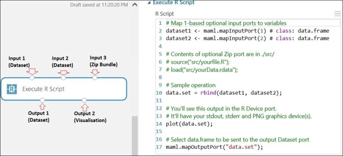
To integrate Python code with ML Studio, you should use the Execute Python Script module, which is the only module available for Python as of writing this book. This module has three input ports and two output ports, as shown in the following screenshot:
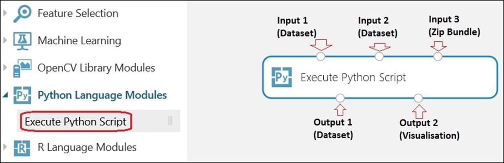
While the first two inputs are datasets, the third one expects a .zip file to be uploaded to ML Studio to import the existing code; you can find more on this in the following sub section. The first output generates a dataset that can be used further in another module and the second output is the generated visualization, Python Device, which you can only right-click on and then click on Visualize to view the generated graph. It supports both the console output as well as the display of PNG graphics using the Python interpreter.
The property section of the module comes with a very basic code editor, where you can write code. It also comes with a basic template of the code. The module must contain a function with the name azureml_main and it should have zero to two parameters. The function must also return aDataFrame object. Let's take a look at the following screenshot which displays the Python code which we need to integrate with the ML Studio:
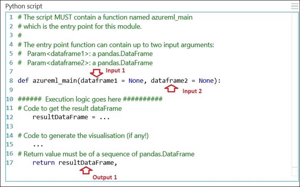
As you can note, the input datasets get converted to Pandas data frames. Connecting a dataset to the input ports is not a must. When an input data port is empty, the corresponding input data frame will be of the value None or null. Note here that the mapping between input ports and function parameters is positional, that is, the first connected input port, if connected, is mapped to the first parameter, dataframe1, of the function and the second input, if connected, is mapped to the second parameter, dataframe2, of the function.
You need to take care of proper indentation for Python code; otherwise, it would result in an error.
Creating visualizations using Python
You can create data visualization using the MatplotLib library or any other library based on it and show it in the browser like any other visualization in ML Studio. However, the visualization created won't be automatically redirected. You have to save them as PNG files for ML Studio to pick it up and make it available through the second output port of the Execute Python Script module. The overall steps to generate data visualization using the MatplotLib library through the module are as follows:
· Change the MatplotLib library backend to agg from the default Qt-based renderer
· Create a figure using the MatplotLib API
· Get the axis and create all plots in the same axis using a MatplotLib API or any other library that uses MatplotLib as a base for plotting, for example, Pandas
· Save the generated figure to a PNG file
Now that you have an overview of how to integrate the Python code, it's time to walk you through an example.
A simple time series analysis with the Python script
The time series is a sequence of data points each having a timestamp associated with it, that is usually measured over a time interval. A simple time series analysis is to find the moving average for the series.
The moving average or simple moving average can be defined as the mean of the previous n number of data in a series. Here, n is the window size. Consider a simple time series data, as the following, where the first column is time, the second column contains value, and the third column calculates the moving average for the window size 3. For each value, its moving average is the average of the previous three values including itself:
|
Time |
Value |
Moving Average = Sum of previous 3 values / 3 |
|
1 |
30 |
- |
|
2 |
25 |
- |
|
3 |
15 |
(15+25+30)/3 = 23.3 |
|
4 |
45 |
(45+15+25)/3 = 28.3 |
|
5 |
55 |
(55+45+15)/3 = 38.3 |
|
6 |
5 |
(5+55+45)/3 = 35.0 |
|
7 |
38 |
(38+5+55)/3 = 32.7 |
|
8 |
13 |
(13+38+5)/3 = 18.7 |
|
9 |
33 |
(33+13+38)/3 = 28.0 |
|
10 |
31 |
(31+33+13)/3 = 25.7 |
We would use the rolling_mean Pandas method to calculate the moving average for the window size 10 to demonstrate the Python script integration We will use the previously mentioned sample time series dataset in ML Studio, add a new column to the dataset, and assign values to it bycalculating the simple moving average for it. Let's take a look at the following screenshot:
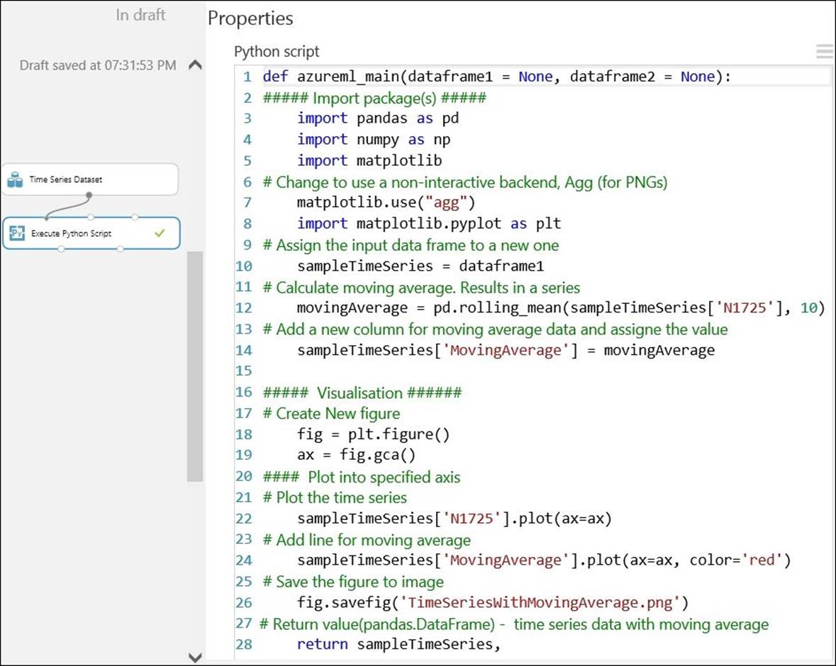
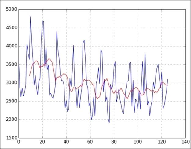
The comments in the code are self-explanatory. If you run your experiment with the preceding code, the first output will get you the modified dataset with the moving average values in the third column and the second output will get you the following visualization, where the red line represents the moving average:
Importing the existing Python code
It may not be always practical to write enough code in a single script box to meet the requirement. Also, there will be scenarios where you would have an already built and tested code or an external library, which you would like to use inside ML Studio. In such scenarios, you can use the third input port (Input3) of the module. You can keep the prebuilt scripts in a folder, ZIP it, and upload it to ML Studio. It will be available in the Saved Datasets section of the modules palette. Then, drag it to the canvas for your experiment and connect it to the third input port, Zip Bundle, of the module. The Azure ML execution framework will unzip it internally during runtime and the contents will be added to the library path of the Python interpreter. This means that the azureml_main entry point function can import these modules directly.
Do it yourself – Python
Add another column to the data frame in the preceding example to moving standard deviation and plot it as another line.
Tip
Use the moving window function rolling_std.
Extending experiments using the R language
Similar to Python, you can also use the R code/script to extend your experiment inside ML Studio. However, unlike Python, you get two modules for R, which are as follows:
· The Execute R Script module
· The Create R Model module
Understanding the Execute R Script module
Similar to the module for Python, the Execute R Script module also has three input ports and two output ports. The property panel for the module comes with an R script editor where you can enter your code, as shown in the following screenshot:
The module comes with a sample script, as you can find in the preceding screenshot. You can use the maml.mapInputPort() method with the port number as argument 1 for Input1, and argument 2 for Input2 to access the input dataset as an R data.frame object.
The third input expects a .zip file to be uploaded to ML Studio to import the existing code. The first output generates a dataset that can be used further in another module and the second output is the generated visualization, R Device, which you can right-click on it and then click onVisualize to view the generated graph. It supports the console output and the display of PNG graphics using the R interpreter. You don't have to take any extra steps to make the visualization available through the second output port of the module, as it would be redirected automatically.
Remember that if you import data that uses CSV or other formats, you have to convert the same to a dataset before using the data in an R module.
A simple time series analysis with the R script
We will use the same time series example, as used previously, but this time, with the R script. We would use functions from an R package called zoo, which is already available in ML Studio. Let's take a look at the following screenshot which displays the code written in R which we are going to integrate with the ML Studio:
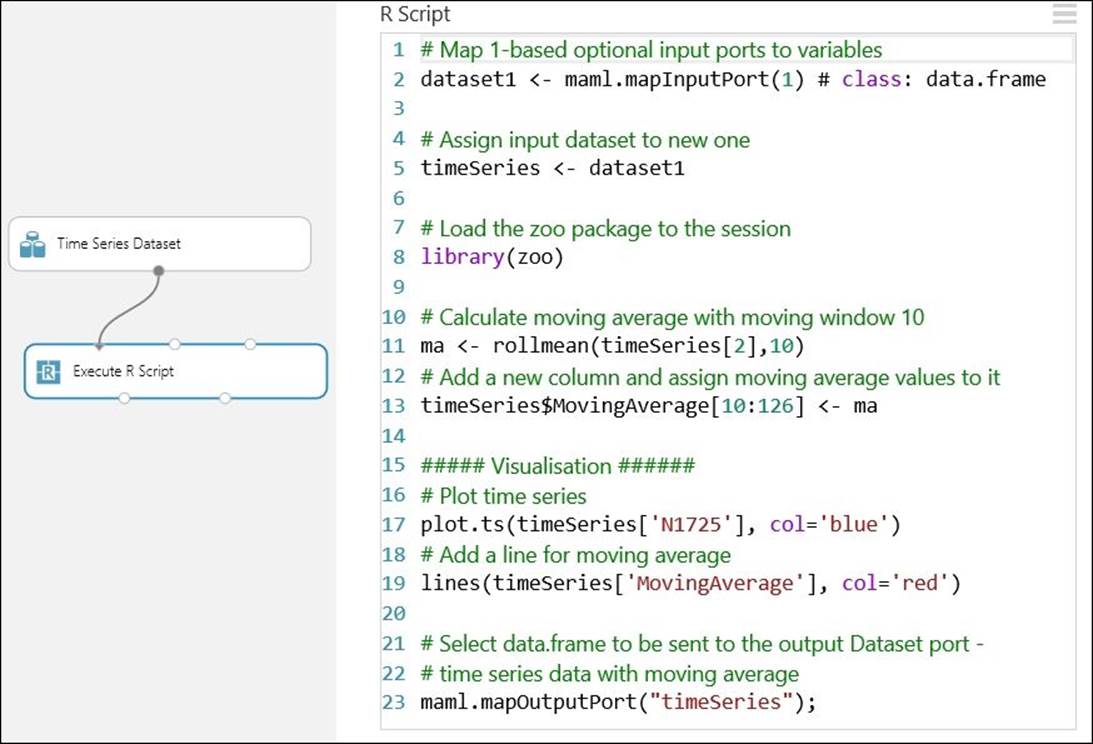
The comments in the code are self-explanatory. However, note that on the line number 13, the new column's moving average values are assigned from the position 10 and to the last position, which is 126 here. As we have taken the moving window as 10, the first nine values for the column would be null or missing.
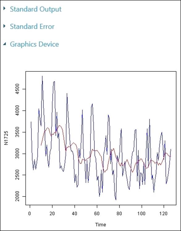
If you run your experiment with the preceding code, the first output will get you the modified dataset with the moving average values in the third column and the second output will get you the following visualization, where the red line represents the moving average:
Importing an existing R code
Like for Python, you can use the third input port (Input3) of the module to import the external code. You can keep the prebuilt scripts in a folder, ZIP it, and then upload it to ML Studio. To upload a ZIP file to your workspace, click on New, click on Dataset, and then select From local fileand the Zip file option. After the upload, the zipped file will be available in the Saved Datasets list. Then, drag it to the canvas for your experiment and connect it to the third input port, Zip Bundle, of the module. All the files present in the ZIP file will be available for use during runtime. If any directory structure is there in the ZIP file, then it would be preserved. The root in the ZIP bundle is referred to as src.
For example, if you have created an R file named myExternalCode.R, zipped it to a file, and uploaded to ML Studio, then you can access it from the script editor for the module, shown as follows:
source("src/myExternalCode.R")
Including an R package
If you want to include any R package that is not available out of the box in ML Studio, then you can ZIP the package and upload it. Usually, R packages are available as downloadable ZIP files. If you have already downloaded and extracted the R package that you are using in your code, you will need to ZIP the package again otherwise upload the original ZIP file for the R package to ML Studio. You need to install the R package as part of the custom code in the Execute R Script module and the package will be installed only for your experiment.
Understanding the Create R Model module
The Create R Model module can be used to create an untrained model using R code. You can build your model using any learner based on an R package or your new implementation.
The module takes the training script and the scoring script, the two user-defined R scripts, as inputs in the property sections based on which, the model will be built.
After you create the model, you can use the Train Model module to train the model on a dataset similar to any other learner in ML Studio. Then, pass it to the Score Model module to use the model to make predictions. You can then save the trained model, create a scoring experiment, and publish it as a web service.
Do it yourself – R
Let's take a look at the following steps to build our own test using R for coding:
1. Add another column to the data frame (in the preceding example) to move the median and plot it as another line.
Tip
Use the moving window function rollmedian.
2. Display all the already installed packages in ML Studio. You may use the following code:
3. data.set <- data.frame(installed.packages())
maml.mapOutputPort("data.set")
Summary
You just completed a very important part of ML Studio in this chapter. You started with an introduction to both R and Python in relation to Azure ML. You explored the importance of why you may need to extend your experiment inside ML Studio using code. Then, you learned how to execute Python scripts and import an already built code inside ML Studio. You applied the same through an example of a simple time series analysis and also created visualization with Python. After Python, you explored the same for R and performed the same tasks of time series analysis and plotted the graph with an R script. ML Studio also comes with another module to build a complete model with R apart from just running a script.
In the next chapter, you will find out how to deploy a model as a web service API from your experiment inside ML Studio, which can be consumed outside.
All materials on the site are licensed Creative Commons Attribution-Sharealike 3.0 Unported CC BY-SA 3.0 & GNU Free Documentation License (GFDL)
If you are the copyright holder of any material contained on our site and intend to remove it, please contact our site administrator for approval.
© 2016-2026 All site design rights belong to S.Y.A.