Microsoft Azure Machine Learning

Chapter 13. Case Study Exercise II

You already solved a real-world classification problem in the previous chapter. In this chapter, we will present a new problem in the form of another case study exercise and we will solve it with a very simple solution. This exercise represents a regression problem.

Like in the previous chapter, it won't present a step-by-step guide with all the details; however, it will provide pointers so that you can solve the problem. This chapter assumes that you have successfully completed all the previous chapters, or already know about Azure ML.

Problem definition and scope

The problem is taken from one of the Kaggle machine learning competitions, where they exposed the datasets with a bit of information and asked the contestants to make a prediction from a test dataset using machine learning techniques. It is about the Africa Soil Property Prediction Challenge. The training dataset contains different measurements of the soil and it is expected that the contestants are able to predict values for five properties of the soil (target variables): SOC, pH, Ca, P, and Sand. Full details regarding this can be found at https://www.kaggle.com/c/afsis-soil-properties/.

For the purpose of this case study, we will choose just one target variable named P and ignore the others. Once you are able to predict one target variable, you can follow the same approach and predict others. So, you should try predicting all the variables by yourself.

The dataset

You can download the dataset and find the description at https://www.kaggle.com/c/afsis-soil-properties/data.

The dataset has been explained in the following term list, as found at the preceding web link:

· PIDN: This is the unique soil sample identifier.

· SOC: This refers to soil organic carbon.

· pH: These are the pH values.

· Ca: This is the Mehlich-3 extractable calcium.

· P: This is the Mehlich-3 extractable phosphorus.

· Sand: This is the sand content.

· m7497.96 - m599.76: There are 3,578 mid-infrared absorbance measurements. For example, the "m7497.96" column is the absorbance at wavenumber 7497.96 cm-1. We suggest you remove spectra CO2 bands, which are in the region m2379.76 to m2352.76, but you do not have to.

· Depth: This is the depth of the soil sample (this has two categories: "Topsoil" and "Subsoil"). They have also included some potential spatial predictors from remote sensing data sources. Short variable descriptions of different terms are provided below and additional descriptions can be found in AfSIS data. The data has been mean centered and scaled.

· BSA: These are the average long-term Black Sky Albedo measurements from the MODIS satellite images (here, BSAN = near-infrared, BSAS = shortwave, and BSAV = visible).

· CTI: This refers to the Compound Topographic Index calculated from the Shuttle Radar Topography Mission elevation data.

· ELEV: This refers to the Shuttle Radar Topography Mission elevation data.

· EVI: This is the average long-term Enhanced Vegetation Index from the MODIS satellite images.

· LST: This is the average long-term Land Surface Temperatures from the MODIS satellite images (here, LSTD = day time temperature and LSTN = night time temperature).

· Ref: This refers to the average long-term Reflectance measurements from the MODIS satellite images (here, Ref1 = blue, Ref2 = red, Ref3 = near-infrared, and Ref7 = mid-infrared).

· Reli: This is the topographic Relief calculated from the Shuttle Radar Topography mission elevation data.

· TMAP and TMFI: These refer to the average long-term Tropical Rainfall Monitoring Mission data (here, TMAP = mean annual precipitation and TMFI = modified fournier index).

Download the training dataset (https://www.kaggle.com/c/afsis-soil-properties/download/train.zip). Note that you may have to create an account to download the dataset. Upload the dataset to ML Studio (for this, refer to Chapter 4, Getting Data in and out of ML Studio, to find details on how to upload a dataset from your local machine to ML Studio).

Data exploration and preparation

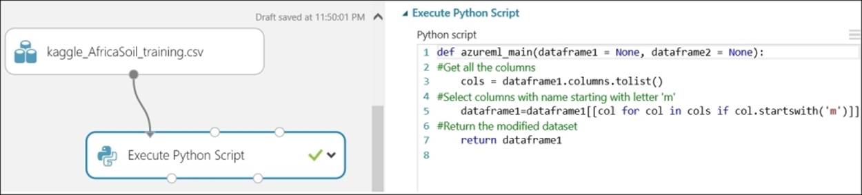
Create a new experiment in ML Studio. Drag the uploaded dataset to the canvas and visualize it. As you can see, it has 1157 rows and 3600 columns. Usually, the data exposed in a Kaggle competition is already cleaned, which saves you the effort of data cleansing, such as dealing with missing values. In ML Studio, you can't see all the columns and rows. There are 3,578 columns that have mid-infrared absorbance measurements and these entire column names start with the letter 'm'. You may like to separate them out. To do so, you can use an Execute Python Scriptmodule with the following code, where the inline comments explain the lines of code. For this, refer to Chapter 10, Extensibility with R and Python, to find the details on how to integrate a Python/R script inside ML Studio:

def azureml_main(dataframe1 = None, dataframe2 = None):

#Get all the columns

cols = dataframe1.columns.tolist()

#Select columns with name starting with letter 'm'

dataframe1=dataframe1[[col for col in cols if col.startswith('m')]]

#Return the modified dataset

return dataframe1

The model in progress may appear as follows:

Alternatively, you can also use an Execute R Script module with R code to achieve the same.

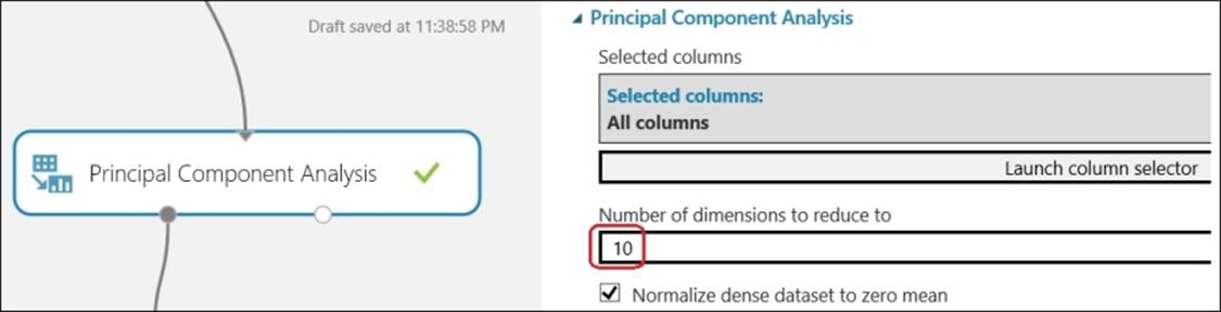
These extracted 3,578 columns are almost impossible to visualize and will take a long time to process in a model, especially when you use the Sweep Parameters module. It would be worthwhile condensing them into a few lines, so they are easier to process. The Principal ComponentAnalysis module would be of great help, as it would extract a given number of the most relevant features from the given features. The Principal Component Analysis (PCA) is a popular technique that takes a feature set and computes a new feature set with reduced dimensionality or a lesser number of features or components; with most of the information contained in the original feature set. The Principal Component Analysis module present in ML Studio takes Number of dimensions to reduce to as input, where you can specify the desired, low number of features.

You may try 10 components (for the Number of dimensions to reduce to option) as its parameter, as shown in the following figure:

You may use another Execute Python Script module or Execute R Script to extract other relevant columns, which are all the columns excluding those that start with 'm' and other target variables (because we are only interested in P). You may also like to exclude PIDN, which is the unique soil sample identifier. Let's take a look at the following screenshot:

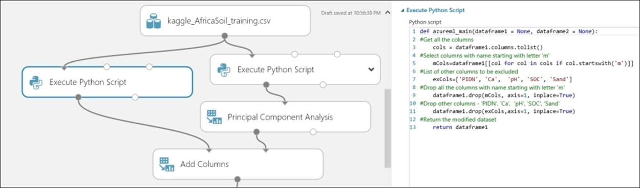
The Python code for the same is as follows:

def azureml_main(dataframe1 = None, dataframe2 = None):

#Get all the columns

cols = dataframe1.columns.tolist()

#Select columns with name starting with letter 'm'

mCols=dataframe1[[col for col in cols if col.startswith('m')]]

#List of other columns to be excluded

exCols=['PIDN', 'Ca', 'pH', 'SOC', 'Sand']

#Drop all the columns with name starting with letter 'm'

dataframe1.drop(mCols, axis=1, inplace=True)

#Drop other columns - 'PIDN', 'Ca', 'pH', 'SOC', 'Sand'

dataframe1.drop(exCols,axis=1, inplace=True)

#Return the modified dataset

return dataframe1

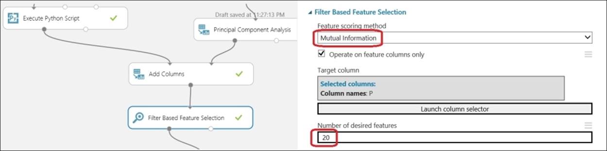
Use the two sets of extracted columns to combine, and make, one dataset using the Add Columns module. By now, you should have a reduced feature set, but you still have to find the most relevant ones. Unnecessary data or noise may reduce the predictive power of a model, so should be excluded. The Filter Based Feature Selection module can identify the most important features in a dataset. You may try the same with a different number of desired features as parameters, and evaluate the performance of the overall model.

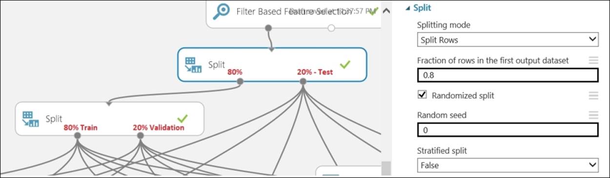
Before you proceed in building the model, you need to prepare train, validate, and test dataset. Let's take a look at the following screenshot:

Model development

After preparing your data, you are not sure which model or regression algorithm would perform well for the problem at hand. Because the target variable P is continuous, you know that it's a regression problem. So, it would be worthwhile trying different algorithms and choosing the best one. You may use the Sweep Parameters module to obtain the optimum parameters for the algorithm. You need to pass three inputs to the Sweep Parameters module: the untrained algorithm, training dataset, and validation dataset. Use the Score modules to score the test data. Use anEvaluate module to compare the two models with the scored data.

You should try different algorithms to choose the best one. The following figure is just for your reference, which shows four algorithms.

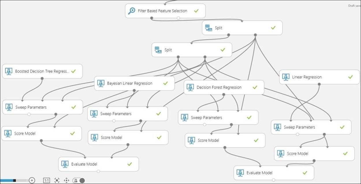
Run the model and find out which algorithm performs the best for you.

Model deployment

After you are happy with a particular model, save it as a trained model and then prepare an experiment for a web service and proceed to deploy the model. Refer to Chapter 11, Publishing a Model as a Web Service, to find the details on how to deploy a model to the staging environment and test it visually in ML Studio.

Chapter 13. Case Study Exercise II