Microsoft Azure Machine Learning

Chapter 5. Data Preparation

In practical scenarios, most of the time you would find that the data available for predictive analysis is not fit for the purpose. This is primarily because of two reasons:

· In the real world, data is always messy. It usually has lots of unwanted items, such as missing values, duplicate records, data in different formats, data scattered all around, and so on.

· Quite often, data is either required in a proper format or needs some preprocessing so that it is ready before we apply machine learning algorithms to it for predictive analysis.

So, you need to prepare your data or transform your data to make it fit for the required analysis. ML Studio comes with different options to prepare your data, and in this chapter, you will explore options to preprocess data for some of the common scenarios and ways to prepare data when necessary modules are not readily available with ML Studio. This chapter aims to familiarize you with these options to provide you with an overview of the practical use of most of these options, which you will find in the subsequent chapters.

Data manipulation

You may need to manipulate data to transform it to the required format. The following are some of the frequently used scenarios and modules available.

Clean Missing Data

Clean missing data and missing values in data are probably the most common problems you need to fix before data analysis. When missing values are present, certain algorithms may not work or you may not have the desired result. So, you need to get rid of the missing values either by replacing them with some logical values or by removing the existing row(s) or column(s).

ML Studio comes with a module, Clean Missing Data, to solve this exact problem. It lets you either remove the rows or columns that have missing values or lets you replace the values in the rows and columns with one of the these: mean, median, mode, custom values, a value that uses the probabilistic form of Principal Component Analysis (PCA), or Multiple Imputation by Chained Equations (MICE). MICE is a statistical technique that updates each column using an appropriate algorithm after initializing the missing entries with a default value. These updates are repeated a number of times and are specified by the Number of Iterations parameter. The default option is to replace the values of the rows and columns with a custom value, where you can specify a placeholder value, such as 0 or NA that is applied to all missing values. You should be careful that the value you specify matches the data type of the column.

The first output of the module is the cleaned dataset while the second one outputs the transformation that is to be passed to the module to clean new data. You can find the Clean Missing Data module under Data Transformation | Manipulation in the module palette.

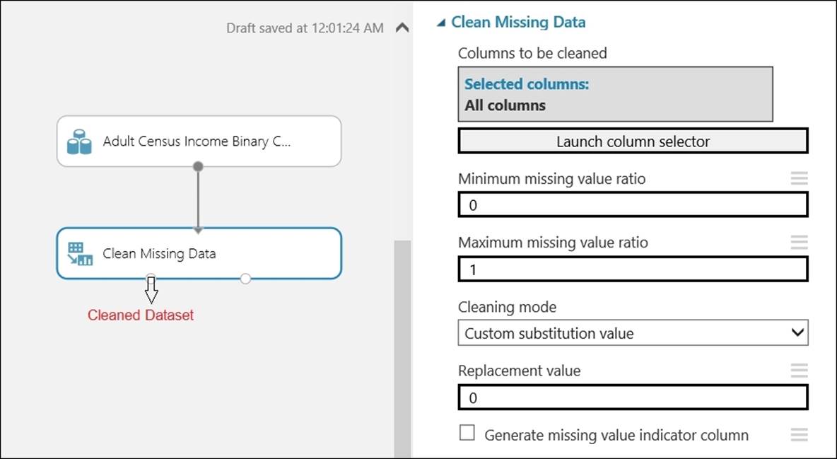
In the last parameter, if you select the check box for Generate missing value indicator column, then it will add a new column for each column containing missing values and will indicate the same for each row it finds a missing value for.

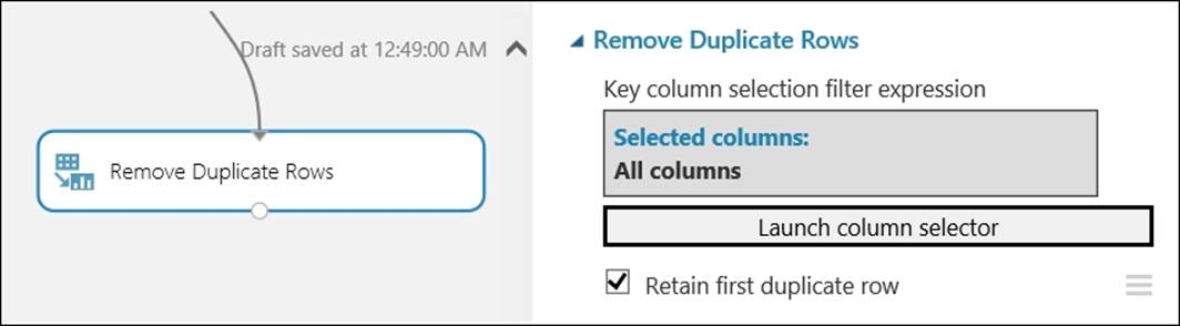
Removing duplicate rows

You use the Remove Duplicate Rows module to remove duplicate rows from the input dataset based on the list of columns you specify. Two rows are considered duplicates if the values of all the included columns are equal. This module also takes an input, that is, the Retain first duplicate row checkbox, as an indicator that specifies whether to keep the first row of a set of duplicates and discard others or to keep the last duplicate row encountered and discard the rest.

Project columns

You can use the Project Columns module when you have to choose specific columns in a dataset for your analysis. Based on your requirements, you can do this either by excluding all columns and including a few columns. Alternatively, you can start with including all the columns and excluding a few.

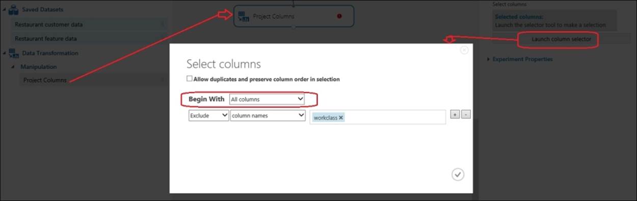
The preceding screenshot illustrates how the Projects Columns module just excludes one column from the given dataset. Also notice that you can tick the checkbox on the top, if you like, to keep the duplicate rows' and columns' order in the selection.

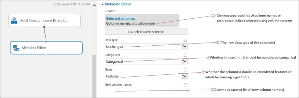
The Metadata Editor module

The Metadata Editor module allows you to change the metadata of one or more columns in a dataset. You can change the following for a given dataset:

· You can change the Datatype of columns; for example, string to integer

· You can change the type of columns to categorical or noncategorical; for example, one column may contain user IDs, which are integers, but you may consider them as categorical

· You can change the consideration of column(s) as features or a label; for example, if one dataset has a column that contains income of a population you are interested making a prediction, you may want to consider it as a label or target variable

· You can change the name of a column

Let's take a look at the following screenshot which explains the various functions provided by the Metadata Editor module:

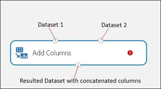
The Add Columns module

The Add Columns module takes two datasets as input and concatenates both by combining all columns from the two datasets to create a single dataset. The resulting dataset will have the sum of the columns of both input datasets.

To add columns of two datasets to a single dataset, you need to keep in mind the following:

· The columns in each dataset must have the same number of rows.

· All the columns from each dataset are concatenated when you use the Add Columns option. If you want to add only a subset of the columns, use the Project Columns module on the result set to create a dataset with the columns you want.

· If there are two columns with the same name, then a numeric suffix will be added to the column name that comes from the right-hand side input.

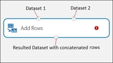
The Add Rows module

The Add Rows module takes two datasets as input and concatenates them by appending the rows of the second dataset after the first dataset.

To add rows of two datasets to a single dataset, you need keep in mind of the following:

· Both the datasets must have the same number of columns

The resulted dataset will have the sum of the number of rows of both the input datasets:

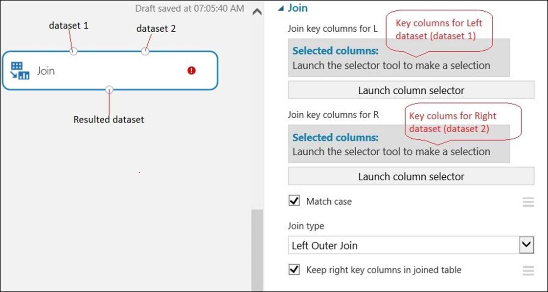
The Join module

The Join module lets you join two datasets. If you are familiar with RDBMS, then you may find it similar to SQL-like join operations; however, no SQL knowledge is required to use it. You can perform the following kinds of join operation:

· Inner Join: This is a typical join operation. It returns the combined rows only when the values of the key columns match.

· Left Outer Join: This returns the joined rows for all the rows from the left-hand side table. When a row in the left-hand side table has no matching rows in the right-hand side table, the returned row contains the missing values of all the columns coming from the right-hand side table.

· Full Outer Join: This returns the joined rows from both datasets with first the result from the Inner Join operation and then appends the rows with a mismatch.

· Left Semi-Join: This returns just the row from the left-hand side table when the values of the key column(s) match.

Splitting data

Quite often, you would need to split your dataset; most commonly, you would need to split a given dataset for analysis into train and test dataset. ML Studio comes with a Split module for this purpose. It lets you split your dataset into two datasets based on a specified fraction. So, if you choose 0.8, it outputs the first dataset with 80 percent of the input dataset, and the rest 20 percent as second output. You also have an option to split the data randomly. You can specify a random seed value other than 0 if you need to get the same result in a random split every time you run it. You can find the Split module under Data Transformation | Sample, and then Split it in the module palette:

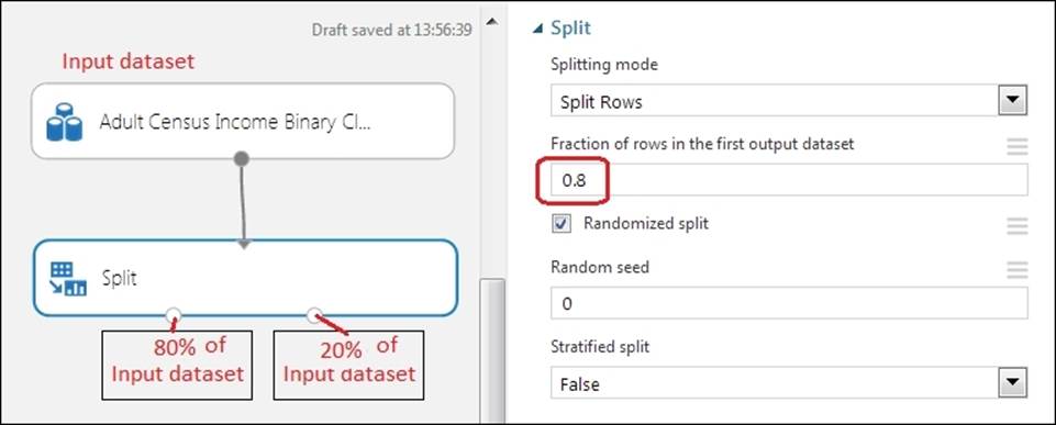
Notice that the last parameter, Stratified split, is False by default, and you make it True only when you go for a stratified split, which means it groups first and then randomly selects rows from each strata (group). In this case, you need to specify the Stratification key column based on which grouping will be made.

You can also specify different Splitting modes as the parameter instead of specifying default split rows, such as:

· The Recommender Split: You can choose this when you need to split data to use it as train and test data in a recommendation model.

· The Regular Expression: You can use this option to specify a regular expression to split the dataset into two sets of rows—rows with values matching the expression and all the remaining rows. The regular expression is applied only to the specified column in the dataset. This splitting option is helpful for a variety of pre-preprocessing and filtering tasks. For example, you can apply a filter on all rows containing the text Social by applying the following regular expression to a string column text Social.

· The Relative Expression: You can use this option and create relational expressions that act as filters on numerical columns; for example, the following expression selects all rows where the values in the column are greater than 2000, such as ColumnName>2000.

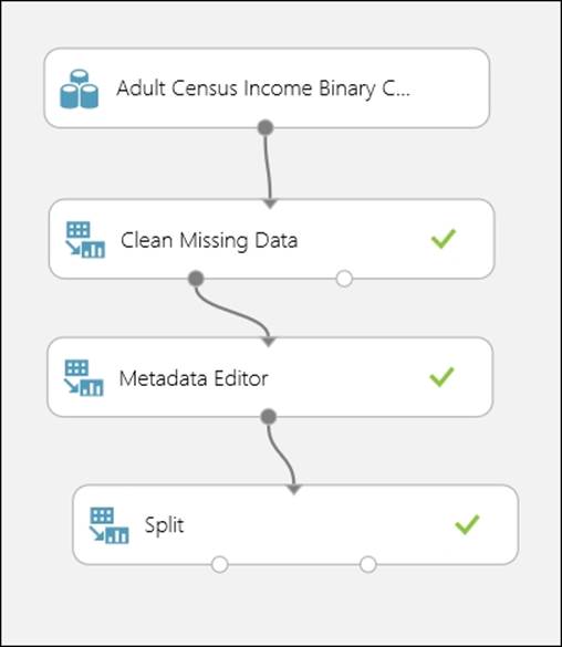
Do it yourself

Start a new experiment and drag the sample dataset, the Adult Census Income Binary Classification dataset, from the module palette under the Saved Datasets group. Then, do the following:

· Visualize the dataset and find out all the columns that have missing values

· Use the Clean Missing Data module to replace the missing values with 0

· On the result dataset of the previously used Metadata Editor module, select all the columns except income and identify them as feature fields

· On the result dataset of the previously used the Split module, split the dataset into 80 percent and 20 percent using the same module

· Run the experiment and visualize the dataset from both the output ports of the Split module

Your experiment may look like the following:

The Apply SQL Transformation module

The Apply SQL Transformation module lets you run a SQL query on the input dataset(s) and get the desired result. You can find it under Data Transformation | Manipulation in the module palette. The module can take one, two, or three datasets as inputs. The dataset coming from input 1 can be referenced as t1. Similarly, you can refer to datasets from input 2 and input 3 as t2 and t3, respectively. On the properties of the module, the Apply SQL Transformation module takes only a parameter as a SQL query. The syntax of the SQL it supports is based on the SQLite standard.

In the following illustration, the module takes data from two datasets, joins them, and selects fewer columns. It also generates calculated columns by applying an aggregation function, AVG.

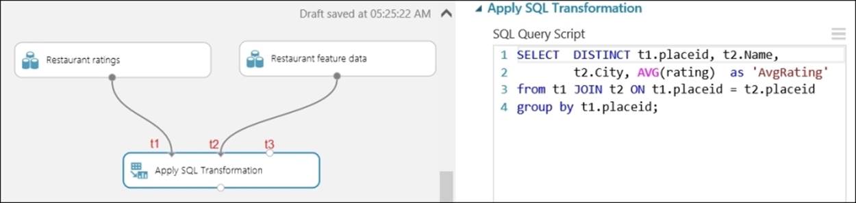
If you are already familiar with SQL, you may find this module very handy for data transformation.

Advanced data preprocessing

ML Studio also comes with advanced data processing options. The following are some of the common options that are discussed in brief.

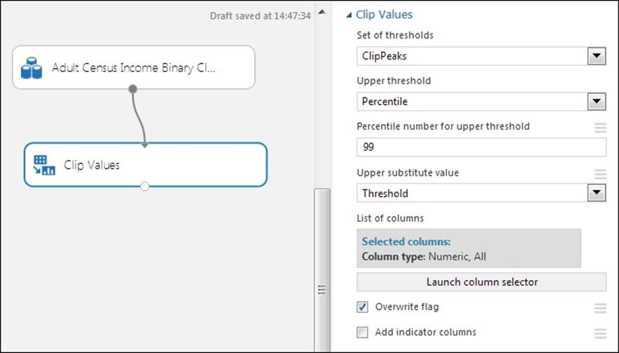
Removing outliers

Outliers are data points that are distinctly separate from the rest of the data. Outliers, if present in your dataset, may cause problems by distorting your predictive model that may result in an unreliable prediction of the data. In many cases, it is a good idea to clip or remove the outliers.

ML Studio comes with the Clip Values module, which detects outliers and lets you clip or replace values with a threshold, mean, median, or missing value. By default, it is applied to all the numeric columns, but you can select one or more columns. You can find it by navigating to Data Transformation | Scale and then Reduce in the module palette.

Data normalization

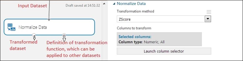
Often, different columns in a dataset come in different scales; for example, you may have a dataset with two columns: age, with values ranging from 15 to 95, and annual income, with values ranging from $30,000 to $300,000. This may be problematic in some cases where certain machine algorithms require data to be in the same scale.

ML Studio comes with the Normalize Data module, which applies a mathematical function to numeric data to make dataset values conform to a common scale; for example, transforming all numeric columns to have values between 0 to 1. By default, the module is applied to all numeric columns, but you can select one or more columns. Also, you can choose from the following mathematical functions:

· Z-Score

· Min-max

· Logistic

· Log-normal

· Tanh

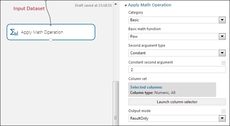
The Apply Math Operation module

Sometimes, you may need to perform a mathematical operation on your dataset as a part of your data preparation. In ML Studio, you can use the Apply Math Operation module, which takes a dataset as input and returns a data table where elements of the selected columns have been transformed by the specified math operation. For unary operations, such as Abs(x), the operation is applied to each of the elements. For binary operations, such as Subtract(x, y), two selections of columns are required and the result is computed over pairs of elements between columns. It gives you a range of mathematical functions grouped under different categories. By default, it is applied to all numeric columns, but you can select one or more columns. You can find it under the Statistical Functions module in the module palette.

Feature selection

Not all features or columns in a dataset have the same predictive power. There are times when data contains many redundant or irrelevant features. Redundant features provide no additional information than the currently selected features, and irrelevant features provide no useful information in any context. So, it's ideal to get rid of redundant or irrelevant features from the dataset before applying predictive analysis.

ML Studio comes with the following two modules for feature selection, which takes an input dataset and result dataset with filtered columns or features.

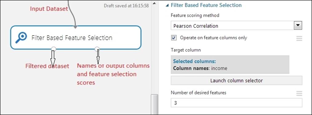
The Filter Based Feature Selection module

The Filter Based Feature Selection module uses different statistical tests to determine a subset of features with the highest predictive power. You can find it under Feature Selection in the module palette. It takes a dataset as input that contains two or more feature columns. The first output is a dataset containing the top N predictive-powered features (columns). The second output is a dataset containing the scores assigned to the selected columns (scalars). This module selects the important features from a dataset based on the following heuristic option that you've chosen:

· Pearson's correlation option

· Mutual information option

· Kendall's correlation option

· Spearman's correlation option

· Chi squared option

· Fisher score option

· Count based option

Pearson's correlation is the default option in the Filter Based Feature Selection module. It works with numeric, logical, and categorical string columns. You should note that all the heuristics or scoring methods don't work with all types of data. So, your selection of the scoring method depends, in part, on the type of data you have. For more details on these scoring methods, you may refer to the product documentation.

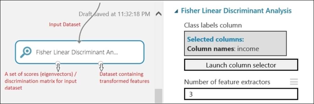
The Fisher Linear Discriminant Analysis module

The Fisher Linear Discriminant Analysis module finds a linear combination of features that characterizes or separates two or more classes of objects or events. The resulting combination is usually used for dimensionality reduction before or after the classification. You can find it underFeature Selection in the module palette.

Data preparation beyond ready-made modules

Though ML Studio comes with many data preprocessing modules, you may come across situations when the available modules don't solve your needs. These are the times you may need to write code in R or Python, run them in ML Studio, and make this part of your experiment. You can find more information on how to write code and extend ML Studio in Chapter 10, Extensibility with R and Python.

It is recommended, as of now, that you do any data preparation inside ML Studio if your data size is within a couple of gigabytes (GB). If you are dealing with more data, then you should prepare your data outside ML Studio, say, using an SQL database or using big data technologies, such as Microsoft's cloud-based Hadoop service HDInsight. Then, you should consume the prepared data inside ML Studio for predictive analytics.

Summary

In any data analysis task, data preparation consumes most of your time. In this chapter, you learned about different data preparation options in ML Studio, starting with exploring the importance of data preparation. Then, you familiarized yourself with some of the very common data transformation tasks, such as dealing with missing values, duplicate values, concatenating rows or columns of two datasets, SQL-like joining datasets, selecting columns in a dataset, and splitting a dataset. You also learned how to apply SQL queries to transform datasets. You explored some of the advanced options of transforming a dataset by applying math functions, normalization, and feature selection.

In the next chapter, you can start applying the machine learning algorithm and, in particular, the regression algorithms that come with ML Studio.