Microsoft Azure Machine Learning

Chapter 6. Regression Models

Finally we are going to start with the machine learning algorithms. You learned earlier that primarily, there are two kinds of supervised machine learning algorithms and regression is one of them. Before you start with different regression algorithms and techniques available with ML Studio, we will try to know more about regression analysis and why it is used.

Understanding regression algorithms

Consider that you live in a locality and you've got the following dataset that has all the transactions of different properties sold in the area along with the property details. Let's take a look at the following table:

Here, D means detached, S means semi detached, T means terraced, and F means flats/maisonettes.

Now, a flat is going to be available on the market of the size; 1,800 square feet. You need to predict the price at which it will be sold. This is a regression problem because you need to predict a number for the target variable. Here, the property price is the target variable and the Property Type and Area are the two features or dependent variables. A target variable in machine learning is also known as a label.

You need to come up with a model that will take the value for the Property Type and Area and output the price. Consider the model as a mathematical function f(Property Type, Area) = Predicted Price.

The actual price at which the property will be sold may or may not be the same as the predicted price. The difference between the actual price and the predicted price is the error. While building a prediction model, you should try to minimize the error so that the predicted value can be as close to the actual value as possible.

Extending the preceding example, you have supposedly built a model and predicted the value for a 1800 square feet flat using the following formula:

f(F, 1800) = $400,000

So, $400,000 is the predicted value, and consider that $410,000 is the actual value at which the property was sold. Then, the error would be Error = $410,000 - $400,000 = $10,000.

Train, score, and evaluate

Before making the prediction, you need to train an algorithm with the example data or training dataset where the target value or the label is known. After training the model, you can make a prediction with the trained model.

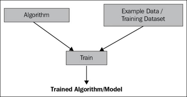
Continuing with the preceding illustration, the trained model may be considered as the mathematical function f to make a prediction.

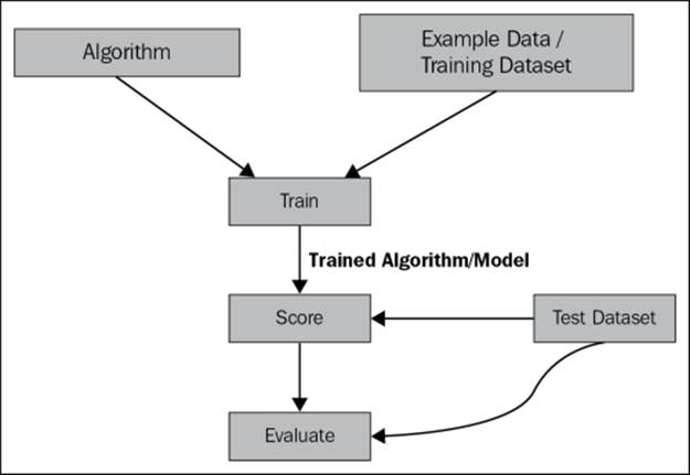
Usually, when you have to build a model from a given dataset, you split the dataset into two sets and use one as a training dataset and the other as a test dataset. After the model is trained with the training data, you use the test dataset to see how the model is performing, that is, how many errors it has.

After the model is trained, you can use the test data to make a prediction or to score. In scoring, the feature values are used and then the target value is predicted. At this point, you are not sure how your model is performing. You need to evaluate it to find out its performance. During evaluation, you take the scored value and the actual value, which is known as you have split your dataset into train and test.

Continuing with the previous illustration, while scoring, you find out that the predicted price of a 1800 square feet flat will be $400,000 and during evaluation, you discover that there is an error of $10,000.

Overall, during experimentation you can follow the given steps:

ML Studio provides different statistics to measure error and performance of your regression model. It also comes with a set of algorithms to experiment with your dataset.

The test and train dataset

Usually, you train an algorithm with your Train dataset and validate or test your model with a test dataset. In practice, most of the time, you are given one dataset. So, you may need to split the given dataset into two and use one as a train and the other as test. Usually, the training set consists of bigger parts and the test set consists of smaller parts, say 70-30 or 80-20. Ideally, while splitting the original dataset, it is split randomly. The Split module in ML Studio solves the purpose well.

Evaluating

Consider the previous illustration of the dataset (refer to table 6.1) as a train dataset and the following as a test dataset:

Consider the actual price and predicted/scored price for the first row as y1 and f1, respectively. So, in the preceding table, we can make out that y1 = 400,000 and f1 = 410,000.

Similarly, we can make out for the second row that y2 = 220,000 and f2 = 210,000.

ML Studio provides the following statistics to measure how a model is performing.

The mean absolute error

The mean absolute error (MAE) is a quantity used to measure how close forecasts or predictions are to the eventual outcomes. It is calculated as the average of the absolute difference between the actual values and the predicted values. Let's take a look at the following figure:

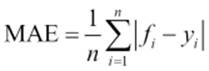
It has the same unit as the original data and it can only be compared between models whose errors are measured in the same units.

The root mean squared error

The root mean squared error (RMSE) is calculated by taking the square root of the average of the square of all the errors (which is the difference between the predicted and actual value). Let's take a look at the following figure:

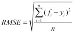
It can only be compared between models whose errors are measured in the same units.

The relative absolute error

The relative absolute error (RAE) is the average of the absolute error relative to the average of the absolute difference of the mean of the actual value and actual values. Let's take a look at the following figure:

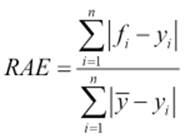
It can be compared between models whose errors are measured in different units.

The relative squared error

The relative squared error (RSE) is the average of the squared difference of the predicted value and the actual value relative to the average of the squared difference, average of the actual value and actual values.

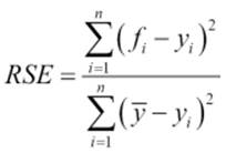
It can be compared between models whose errors are measured in different units.

The coefficient of determination

The coefficient of determination R2 summarizes the explanatory power of the regression model. If the regression model is perfect, though not practical, R2 is 1.

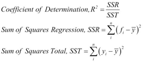
The coefficient of determination can also be interpreted as the percent of the data that fits in the model. For example, if R2 = 0.7950, then 79 percent of the total variation in y can be explained by the linear relationship between features and y, the response variable (or the target variable).

So, for your model, the closer R2 is to 1, the better it is. For all other the error statistics, the less the value, the better it is.

Linear regression

Linear regression is one of the regression algorithms available in ML Studio. It tries to fit a line to the dataset. It is a popular algorithm and probably the oldest regression algorithm. We will use it to train the model to make prediction for one of the sample datasets available: automobile price data (Raw). This dataset is about automobiles distinguished by their make and model and other features. It also includes price. More information on the dataset can be found at https://archive.ics.uci.edu/ml/datasets/Automobile.

We will use price as a label or the target variable here. So, given the automobile features, you need to predict the price of the automobile.

Go to ML Studio and create a new experiment. Then, expand Saved Datasets in the modules palette to the left of the screen. Drag the Automobile price data (Raw) module to the canvas.

Then, expand Data Transformation and then Sample and Split in the modules palette and drag the Split module to the canvas. Set the Fraction of rows parameter in the first output dataset to 0.8 and leave the others to their default values. You are splitting the dataset so that 80 percent of the data will be used to train and the other 20 percent will be used for test.

After you are ready with your train and test data, drag the Train module to canvas. Type train in the search box in the modules palette to the left of the screen and when the Train module appears, drag it to the canvas. Then, join the first output of the Split module to the second input of theTrain module. Now, you need to select the column of the dataset that will be your target variable, or for which you will train a model to make a prediction. In our case, price is the target variable or label for which you are going to make a prediction.

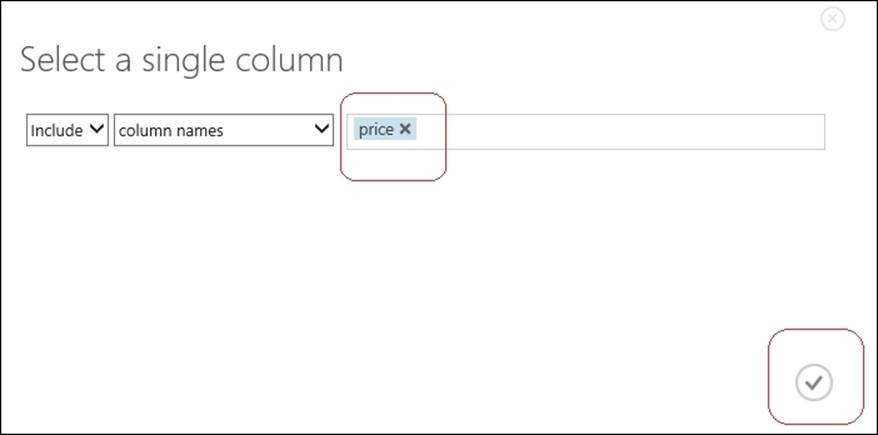
Select the Train module by clicking on it, expand the properties pane to the right of the screen, and click on the Launch column selector option.

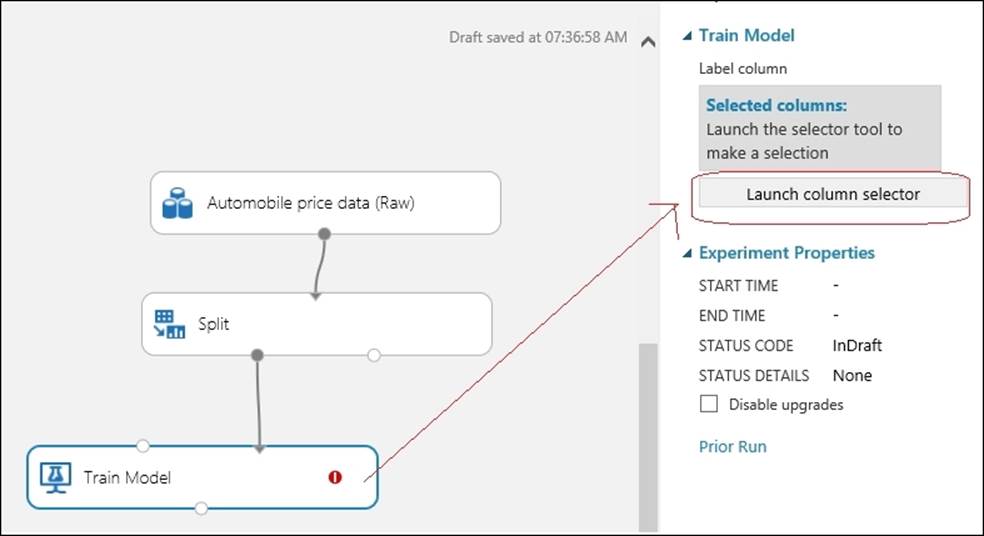
Then, the pop up to select a column will appear. Type price in the textbox to the right of the screen and click on the tickbox to select the column.

Likewise, drag the Linear Regression module to the canvas. Type linear in the search box in the modules palette to the left of the screen and when the module appears, drag it to the canvas.

Then, select the Linear Regression module and leave the property values at default. Use 0 for the Random number seed option. The Random number seed option is used to generate a random number that is used for reproducible results.

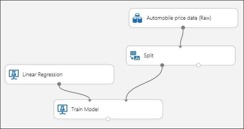
Now, join the output of the Linear Regression module to the first input port of the Train module. It should look like something similar to the following screenshot:

Next, drag the Score Model and the Evaluate Model modules to the canvas.

The Score Model will generate the predicted price value for the test dataset using the trained algorithm. So, it takes two inputs: first, the trained model and second, the test dataset. It generates the scored dataset that contains the predicted values. The Evaluate Model takes a scored dataset and generates an evaluation matrix. It can also take two scored datasets so that you can compare two models side by side.

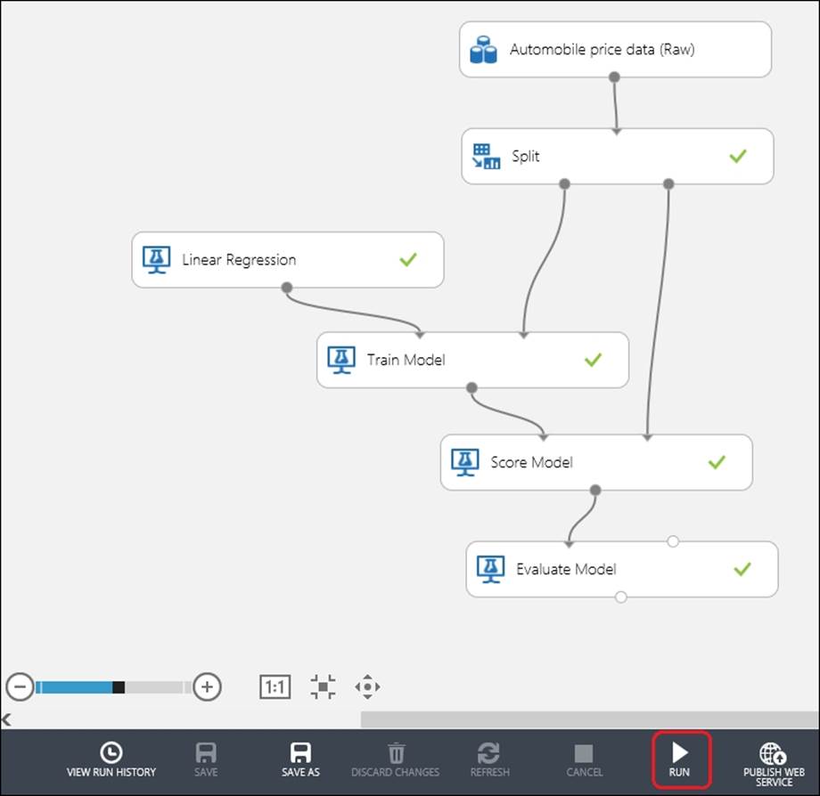
Connect the output of the Train Model to the first input of the Score Model and the second output of the Split module to the second input. Then, connect the output of the Score Model to the first input of the Evaluate Model.

The complete model may look as follows. Now, click on the Run button to run the experiment.

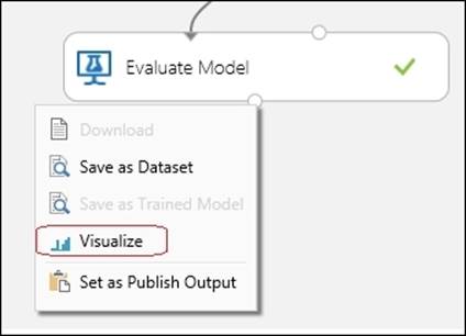
After the run is complete and you see the green tick mark on all the module boxes, you can see the evaluation matrix to find out how your model is performing. To do so, right-click on the output of the Evaluate Model and select the Visualize option by clicking on it.

The following popup displays the Evaluation Results graph, as shown in the following screenshot:

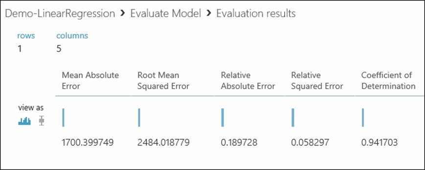
As you can see, Coefficient of Determination is 0.941703, which is decent and the model seems to be performing well.

If you had noticed, you have trained this linear regression model using the Ordinary Least Squared method. You could also have used the Online Gradient Descent with proper parameters, such as the learning rate and number of epochs (iterations). While working with a large dataset, this method can be quite useful as it scales very well. However, working with a few thousand data points in a dataset's Ordinary Least Squared method might be the choice for you as it is simple and easy to train (with a few parameters to choose from).

To keep it simple, in the preceding and following illustrations in this chapter, we have started modeling without initial data preparation, such as removing missing values or choosing the right set of columns or features. In practice, you should always do initial data preparation before training with a dataset. Again, some algorithms require data to be in the proper format to generate the desired result.

Optimizing parameters for a learner – the sweep parameters module

To successfully train a model, you need to come up with the right set of property values for an algorithm. Most of the time, doing this is not an easy task. First, you need to have a clear understanding of the algorithm and the mathematics behind it. Second, you have to run an experiment many times, trying out many combinations of parameters for an algorithm. At times, this can be very time consuming and daunting.

For example, in the same preceding example, what should be the right value for L2 regularization weight? It is used to reduce overfitting of the model. A model overfits when it performs well on a training dataset, but performs badly on any new dataset. By reducing overfitting, you generalize the model. However, the problem here is that you have to manually adjust this L2 regularization weight, which can be done by trying different values, running the experiment many times, and evaluating its performance in each run.

ML Studio comes with a sweet solution to this in the form of the Sweep Parameters module. Instead of a Train Model module, you can use the Train Model module to generate a trained model optimized with the right set of parameters or property values. The following screenshot describes its inputs and outputs:

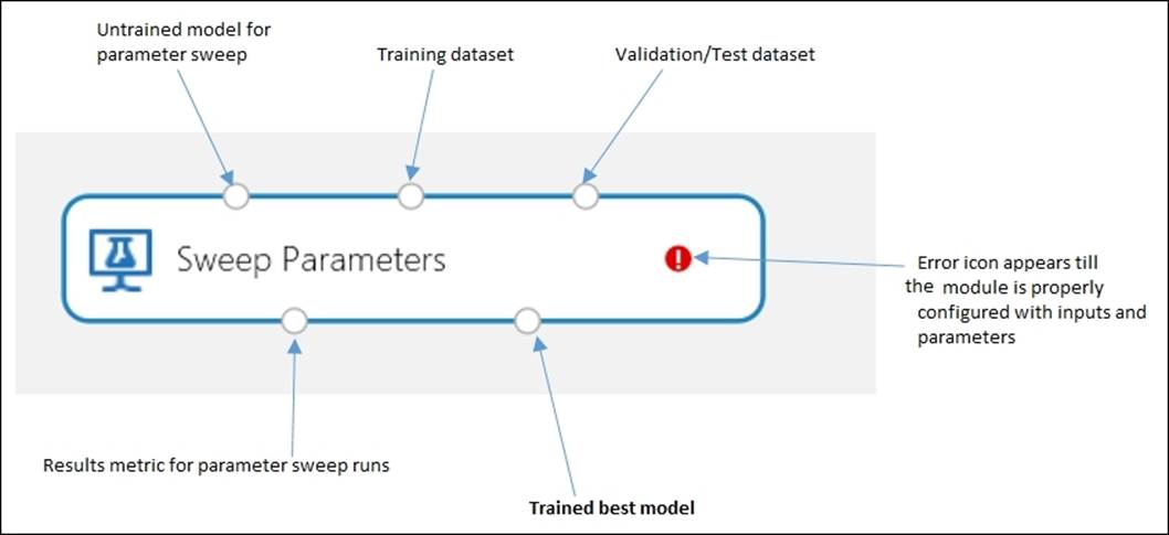
You need to specify a parameter sweeping mode as a parameter of this module. You have two options to specify the parameter of sweeping mode, they are as follows:

· Entire grid: This option is useful for cases where you don't know what the best parameter settings might be and want to try many parameters. It loops over a grid predefined by the system to try different combinations and identify the best learner.

· Random Sweep: Alternatively, you can choose this option and specify the maximum number of runs that you want the module to execute. It will randomly select parameter values over a range of a limited number of sample runs. This option is suggested when you want to increase the model's performance using the metrics of your choice and conserve computing resources.

You also need to choose a target or label column along with specifying a value for metric to measure the performance of regression, which can be one of the five evaluation matrices, for example, the root mean squared error. While working on a regression problem, you may ignore the parameter setting for classification.

The decision forest regression

Decision forest, or random forest as it is widely known, is a very popular algorithm. Internally, it constructs many decision trees and then ensembles them as a forest. Each decision tree generates a prediction and in the forest, the predicted values of each tree is averaged out. It works well even in the case of noisy data.

However, to train a decision forest, you need to set the right parameters, for example, the number of decision trees. We will now train a decision forest and optimize its parameters with the Sweep Parameters module.

As in the previous case, create a new experiment and give a name to it. Then, do the same steps and expand Saved Datasets in the modules palette to the left of the screen. Drag the Automobile price data (Raw) module to the canvas.

Then, expand Data Transformation and Sample and Split in the modules palette and drag the Split module to the canvas. Set the Fraction parameter of the rows in the first output dataset to 0.8 and leave the others to their default values. You are splitting the dataset so that 80 percent of the data will be used for train and the other 20 percent will be used as test.

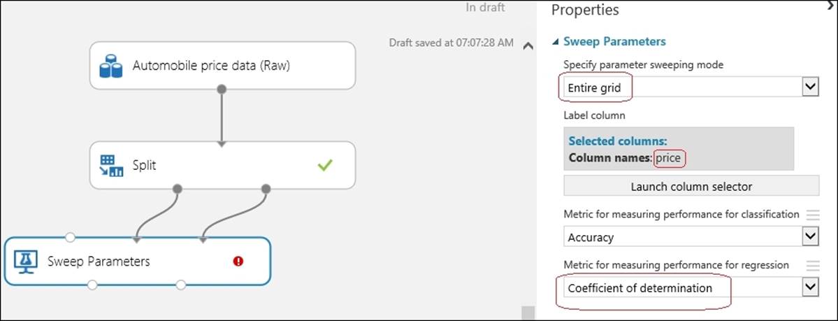
Type Sweep in the search box in the modules palette to the left of the screen and when the Sweep Parameters module appears, drag it to the canvas. Then, join the first output of the Split module to the second input of the Sweep Parameters module and join the second output of the Splitmodule to the third input of the Sweep Parameters module.

Now, you need to set the column of the dataset that is your target or label column for which you will train a model to do a prediction. In our case, price is the target variable or label for which you are going to make a prediction. Also, set the sweeping mode to Entire grid and Metric for measuring performance for regression to Coefficient of determination.

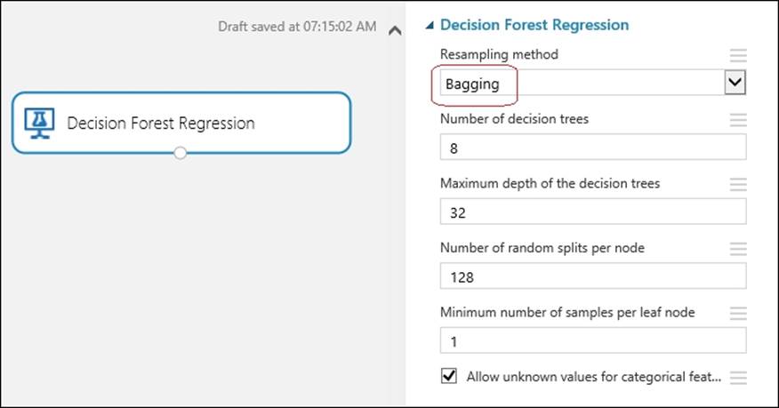
Likewise, drag the Decision Forest Regression module to the canvas. Type Decision Forest in the search box in the modules palette to the left of the screen and when the module appears, drag it to the canvas. Set the Resampling method property to Bagging and leave the rest with their default values, as you can see in the following screenshot:

Then, connect the only output of the Decision Forest Regression module to the first input of the Sweep Parameters module.

Next, drag the Score Model and Evaluate Model to the canvas. Connect the second output of the Sweep Parameters module to the first input of the Score Model and connect the second output of the Split module to the second input of the Score Model. Then, connect the output of theScore Model to the first input of the Evaluate Model.

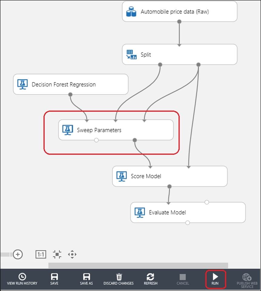
Now, run the experiment and after completion, visualize the output of the Evaluate Model to know the performance of the model.

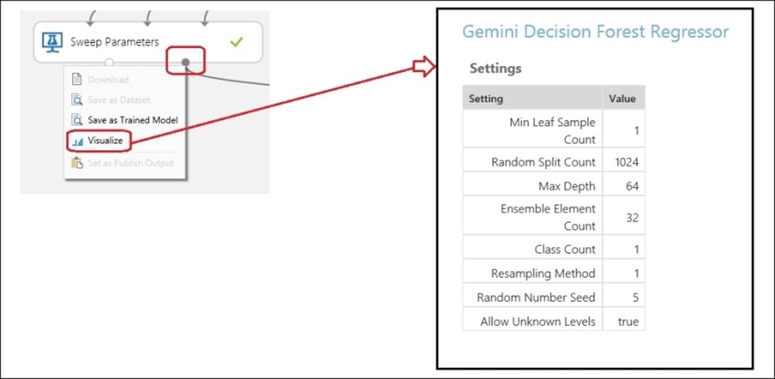
If you are interested to know about the optimum parameters for the Decision Forest Regression module obtained by the Sweep Parameters module, then right-click on the Sweep Parameter module's output port and click on Visualize. In the preceding case, it looked as follows:

The train neural network regression – do it yourself

Neural network is a kind of machine learning algorithm inspired by the computational models of a human brain. For regression, ML Studio comes with the Neural Network Regression module. You can train this using the Sweep Parameters module. First, try to train it without the Sweep Parameters module (with the Train module) with default parameters for Neural Network Regression and then train it with the Sweep Parameters module. Note the improvement in performance of the model.

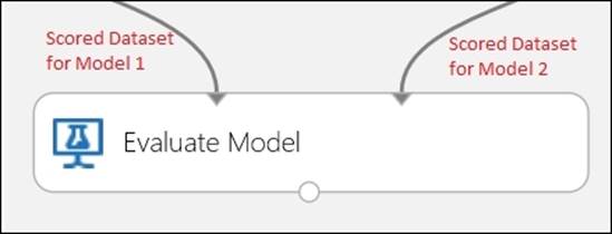
Comparing models with the evaluate model

With the Evaluate Model, you can also compare two models side by side in the same experiment. The two input ports of the module can take the output from the two Score modules and generate the evaluation matrix to compare the output from the two inputs that the module accepts. As shown in the following screenshot:

Comparing models – the neural network and boosted decision tree

The Boosted Decision Tree Regression module is another regression algorithm that comes with ML Studio. It is an ensemble model like decision forest, but is a bit different.

Here, we will use both the Boosted Decision Tree Regression and Neural Network Regression modules in the same experiment and compare both using the Evaluate Model. We will use the Sweep Parameters module in both cases, to train the algorithm.

Create a new experiment and drag the same sample dataset—the Automobile price data (Raw) module. Then, use the two algorithms with the same training dataset (80 percent) and also score using the other 20 percent. The constructed model may look like the following:

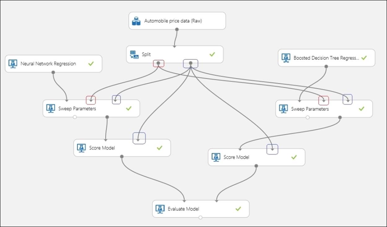
While the connections are straight-forward and intuitive, the connection for the Sweep Parameters module for both the cases might be confusing. Note that the inputs with the red circles are coming from the same output of the Split module also marked with a red circle. So, the two Sweep Parameters modules accept the same training data, but different algorithms to train with. Also, note the input ports marked with the blue circle coming from the same output port of the Split module also marked with a blue circle.

After you run the experiment successfully, all the boxes will have a green tick mark. Then, right-click on the output port of the Evaluate Model to find the comparison metrics for both the algorithms. Let's take a look at the following screenshot:

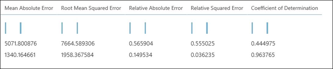
The first row in the preceding screenshot shows the metrics for the model connected to the first input of the Evaluate Model and in this case, it shows the Neural Network Regression module and the second row for the second model: the Boosted Decision Tree Regression module. You know that for better performing models, error values should be as less as possible and the coefficient of determination should be as close as possible to 1, which means that the higher it is the better. As you will find, the Boosted Decision Tree outperforms the Neural Network for this dataset on every evaluation statistic, for example, the Coefficient of Determination is 0.963765 versus 0.444975. Similarly, the relative absolute error is much less for the Boosted Decision Tree as compared to others. If you have to choose between these two models, then in this case, you will naturally choose the Boosted Decision Tree. Because we have not set a random number seed, your results (figures) may be slightly different; however, overall, it doesn't make any difference.

Here, you compared only two models. In practice, you can and should compare as many models as possible on the same problem to find out the best performing model among them.

Other regression algorithms

Azure ML comes with a bunch of popular regression algorithms. This section briefly describes other algorithms available (at the time of writing of this book) that we have not discussed so far:

· The Bayesian Linear Regression Model: This model uses Bayesian Inference for regression. This may not be difficult to train as long as you get the regularization parameter right, which may fit a value such as 0.1, 0.2, and so on.

· The Ordinal Regression Model: You use this when you have to train a model for a dataset in which the labels or target values have a natural ordering or ranking among them.

· The Poisson Regression: It is a special type of regression analysis. It is typically used for model counts, for example, modeling the number of cold and flu cases associated with airplane flights or estimating the number of calls related to an event or promotion and so on.

No free lunch

The No Free Lunch theorem is related to machine learning and it popularly states the limitation of any machine learning model. As per the theorem, there is no model that fits the best for every problem. So, one model that fits well for one problem in a domain may not hold good for another. So in practice ,whenever you are solving a problem, you need to try out different models and experiment with your dataset to choose the best one. This is especially true for supervised learning; you use the Evaluate Model module in ML Studio to assess the predictive accuracies of multiple models of varying complexity to find the best model. A model that works well could also be trained by multiple algorithms, for example, linear regression in ML Studio can be trained by Ordinary Least Square or Online Gradient Descent.

Summary

You started the chapter by understanding predictive analysis with regression and explored the concepts of training, testing, and evaluating a regression model. You then proceeded to carry on building experiments with different regression models, such as linear regression, decision forest, neural network, and boosted decision trees inside ML Studio. You learned how to score and evaluate a model after training. You also learned how to optimize different parameters for a learning algorithm with the Sweep Parameters module. The No Free Lunch theorem teaches us not to rely on any particular algorithm for every kind of problem, so in ML Studio you should train and evaluate the performance of different models before finalizing a single one.

In the next chapter, you will explore another kind of unsupervised learning called classification and you will explore the different algorithms available with ML Studio.