Microsoft Azure Machine Learning

Chapter 7. Classification Models

Classification is another kind of supervised machine learning. In this chapter, before getting into the details of building a classification model using ML Studio, you will start with gaining the basic knowledge about a classification algorithm and how a model is evaluated. Then, you will build models with different datasets using different algorithms.

Understanding classification

Consider you are given the following hypothetical dataset containing data of patients: the size of the tumor in their body, their age, and a class that justifies whether they are affected by cancer or not, 1 being positive (affected by cancer) and 0 being negative (not affected by cancer):

Here, the patients are classified as cancer-affected or not. A new patient comes in at the age 17 and is diagnosed of having a tumor the of size 149. Now, you need to predict the classification of this new patient based on the previous data. That's classification for you as you need to predict the class of the dependent variable; here it is 0 or 1—you may also think of it as true or false.

For a regression problem, you predict a number, for example, the housing price or a numerical value. In a classification problem, you predict a categorical value, though it may be represented with a number, such as 0 or 1.

You should not be confused between a regression and classification problem. Consider a case where you need to predict the housing price not as a number, but as categories, such as greater than 100K or less than 100K. In this case, though you are predicting the housing price, you are indeed predicting a class or category for the housing price and hence, it's a classification problem.

You build a classification model by training an algorithm with the given training data. In the training dataset, the class or target variable is already known.

Evaluation metrics

Suppose that you have built a model and trained a classification algorithm with the dataset in Table 7.1 as the training data. Now, you are using the following table as your test data. As you can see, the last column has the predicted class.

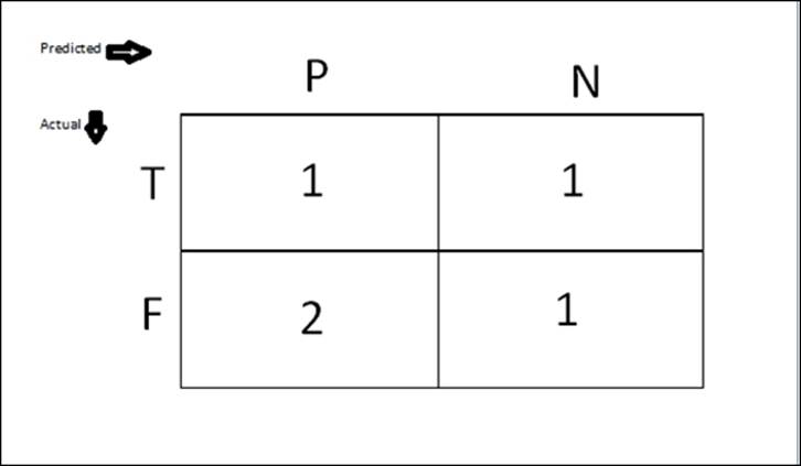
True positive

This is the number of times an actual class was positive and was predicted as positive. For example, the patient is actually affected by cancer and the model is also predicted positive.

In our preceding example, there is one instance where the Actual Class = 1 and Predicted Class = 1. So here, TP = 1.

False positive

This is the number of times an actual class was negative and was predicted as positive. For example, the patient is actually not affected by cancer but the model is predicted as positive.

In our preceding example, there are two instances where the Actual Class = 0 and Predicted Class = 1. So here, FP = 2.

True negative

This is the number of times an actual class was negative and it was predicted as negative. For example, the patient is actually NOT affected by cancer and the model also predicted it as negative.

In our preceding example, there was one instance where the Actual Class = 0 and Predicted Class = 0. So here, TN = 1.

False negative

This is the number of times an actual class was positive but was predicted as negative. For example, the patient is actually affected by cancer but the model predicted it as negative.

In our preceding example, there was one instance where the Actual Class = 1 and Predicted Class = 0. So here, FN = 1.

The following table shows TP, TN, FP, and FN in a matrix:

Accuracy

It is the proportion of a true prediction to the total number of predictions. While true prediction is TP + TN, the total number of predictions are of the size of a test dataset, which is also TP + TN + FP + FN. So, accuracy can be represented in a formula as follows:

Accuracy = (TP + TN) / (TP + TN + FP + FN)

So in our example, Accuracy = (1 + 1) / (1 + 1 + 2 + 1) = 2/5 = .4.

Accuracy can also be represented as a percentage of the prediction that was accurate. So, in our example, accuracy is 40 percent.

Note

Note that the preceding figures are just for illustration of how the calculation is done. In practice, when you build a model, it should have an accuracy of more than 50 percent; otherwise, the model is no good because even a random trial will have 50 percent accuracy.

Precision

The positive predictive value or precision is the proportion of positive cases that the model has correctly identified. Precision can be represented in the formula form, as follows:

Precision = TP / (TP + FP)

So in our example, Precision = 1 / ( 1+1) = 1/2 = .5.

Recall

Sensitivity or recall is the proportion of actual positive cases that are correctly identified. The formula for recall is:

Recall = TP / (TP + FN)

So in our example, Recall = 1 / (1 +2) = 1/3 = .33.

The F1 score

The F1 Score can be defined as a formula, as follows:

F1 = 2TP / (2TP + FP + FN)

The F1 Score can also be defined in terms of precision (P) and recall (R), as follows:

F1 = 2PR/(P+R)

So in our example, F1 = (1 * 2) / {(1 * 2) + 2 + 1 } = 2/ (2 + 2 +1) = 2/5 =.4.

Threshold

Threshold is the value above which the threshold belongs to the first class and all the other values belong to the second class. For example, if the threshold is 0.5, then any patient who has scored more than or equal to 0.5 is identified as sick; otherwise, the patient is identified as healthy. You can think of threshold as probability. To illustrate, if there is a probability of 80 percent or .8 percent that it may rain today, then you may predict that rain for today is true. Similarly, if it is less than .8, then you can predict that it won't rain. So your prediction would depend on the threshold here.

Understanding ROC and AUC

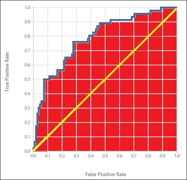
The receiver operating characteristics (ROC) graph is a two-dimensional graph in which the true positive rate (TP) is plotted on the y axis and the false positive rate (FP) is plotted on the x axis. An ROC graph depicts the relative tradeoffs between benefits (true positives) and costs (false positives).

The Area Under the Curve (AUC) is a portion of the area under the ROC curve of the unit square; its value will always be between 0 and 1, where 1 is the best case or everything is predicted correctly. However, because random guessing produces the diagonal line between (0, 0) and (1, 1), which has an area of 0.5, no realistic classifier should have an AUC less than 0.5. AUC is often used as a measure of quality of a classification model.

In the following diagram, the blue curve shows the ROC while the area painted in red shows the AUC. The yellow painted diagonal line represents the random guessing:

Motivation for the matrix to consider

While choosing an algorithm for your model, you will have to rely on the preceding metrics that are defined. Often, one metric may not be sufficient to take a decision. To start with, you may look at accuracy, but at times it might be deceptive. Consider a case where you are making a prediction for a rare disease where in reality, 99 percent negative cases and 1 percent of positive cases appear. If your classification model predicts all the cases as true negatives, then the accuracy is still 99 percent. In this case, the F1 score might be useful as it would give you a clear picture. AUC might also be useful for this.

Consider another scenario. Let's stick to our disease prediction example. Suppose you are predicting whether a patient has cancer or not. If you predict a false case (where the patient is NOT affected by the disease) as true, it's a false positive case. In the practical scenario, after such a prediction, the patient will have further medical tests to manually declare as not affected by cancer. However, if you have a predicted true case (where the patient is actually affected by the disease) as false, then it's a false negative case. In practical scenarios, after such a prediction, the patient is left free and allowed to go home without medication. This might be dangerous as the patient might lose life. You may never like to make such a prediction. In such a scenario, as in this story, you may reduce the threshold value to reduce the chance of releasing any true positive cases. Hence, it would result in higher recall and lower precision.

In the scenario opposite to the preceding, say you have a classification model to predict the fraud for an online transaction. Here, predicting a case as fraud, (which is actually not—a case of false positive) may result in poor customer satisfaction. So in this scenario, you may increase the threshold value and hence it would result in higher precision and lower recall.

As you may find from the preceding definition, the F1 score is a balanced approach for measurement, which involves both precision and recall.

When you are not too worried about precision and recall or you are not so sure about them, you can just follow the value of AUC (the higher the better). Many find AUC the best way to measure the performance of a classification model. AUC also provides a graphical representation. However, it is always a good idea to take a note of more than one metric.

Training, scoring, and evaluating modules

As with regression problems, which you saw in the previous chapter, with classification problems, you can start with an algorithm and train it with data. You can then score ideally with the test data and evaluate the performance of the model.

Navigate to the Train | Score | Evaluate option on the screen.

The Train, Score, and Evaluate modules are the same as you used for regression. The Train module requires the name of the target (class) variable. The Evaluate module generates evaluation metrics for classification.

If you want to tune parameters of an algorithm by parameter sweeping, you can use the same Sweep Parameters module.

Classifying diabetes or not

The Pima Indians Diabetes Binary Classification dataset module is present as a sample dataset in ML Studio. It contains all of the data of female patients of the same age belonging to Pima Indian heritage. The data includes medical data, such as glucose and insulin levels, as well as lifestyle factors of the patients. The columns in the dataset are as follows:

· Number of times pregnant

· Plasma glucose concentration of 2 hours in an oral glucose tolerance test

· Diastolic blood pressure (mm Hg)

· Triceps skin fold thickness (mm)

· 2-hour serum insulin (mu U/ml)

· Body mass index (weight in kg/(height in m)^2)

· Diabetes pedigree function

· Age (years)

· Class variable (0 or 1)

The last column is the target variable or class variable that takes the value 0 or 1, where 1 is positive or affected by diabetes and 0 means that the patient is not affected.

You have to build models that could predict whether a patient has diabetes or tests positive or not.

Two-class bayes point machine

Two-class Bayes Point Machine is a simple-to-train yet powerful linear classifier. We will build our first classification model using it.

Start a new experiment. On the left-hand side module palette on the screen, expand the Saved Datasets option, scroll down, and drag the Pima Indians Diabetes Binary Classification dataset module to the canvas. Alternatively, you could just type pima in the search box to locate the module and then drag it.

Right-click on its output port and click on the Visualize option to explore the dataset. You can note that it now has 768 rows and 9 columns.

You have to split this dataset into two to prepare your train and test dataset. So, drag the Split module to the canvas and connect the output of the dataset module to the input of the Split module. Set 0.8 as the parameter; the Fraction of rows option is the first output dataset that splits itself in the ratio of 80:20 to get your train and test dataset, respectively.

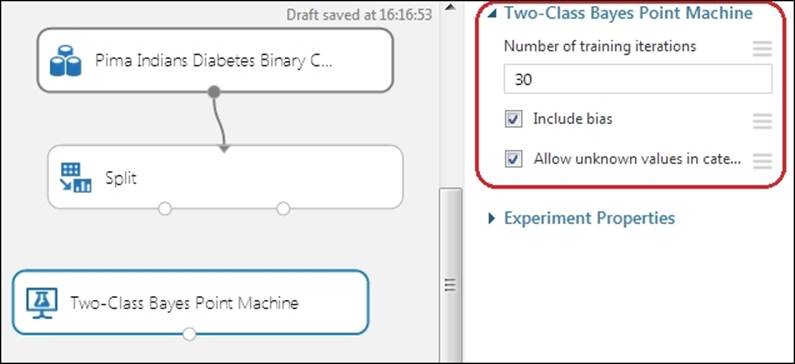
Drag the Two-Class Bayes Point Machine module, which you can find by navigating to Machine Learning | Initialize Model | Classification on the left-hand side module's palette to the canvas.

This module has three parameter values to set. The Number of training iterations module is the value that decides the number of times the algorithm iterates over the dataset. The default value 30 is sufficient most of the time. The Include bias checkbox if ticked or set to true, adds a constant feature or bias to each instance in training and prediction. The default value is true and it is required to be true most of the time. The last parameter, Allow unknown values in categorical features, if ticked or set to true, creates an additional level for each categorical column. Any levels in the test dataset not available in the training dataset are mapped to this additional level. Unless you are doing the required data preprocessing, it is suggested that you tick this or leave it at the default value.

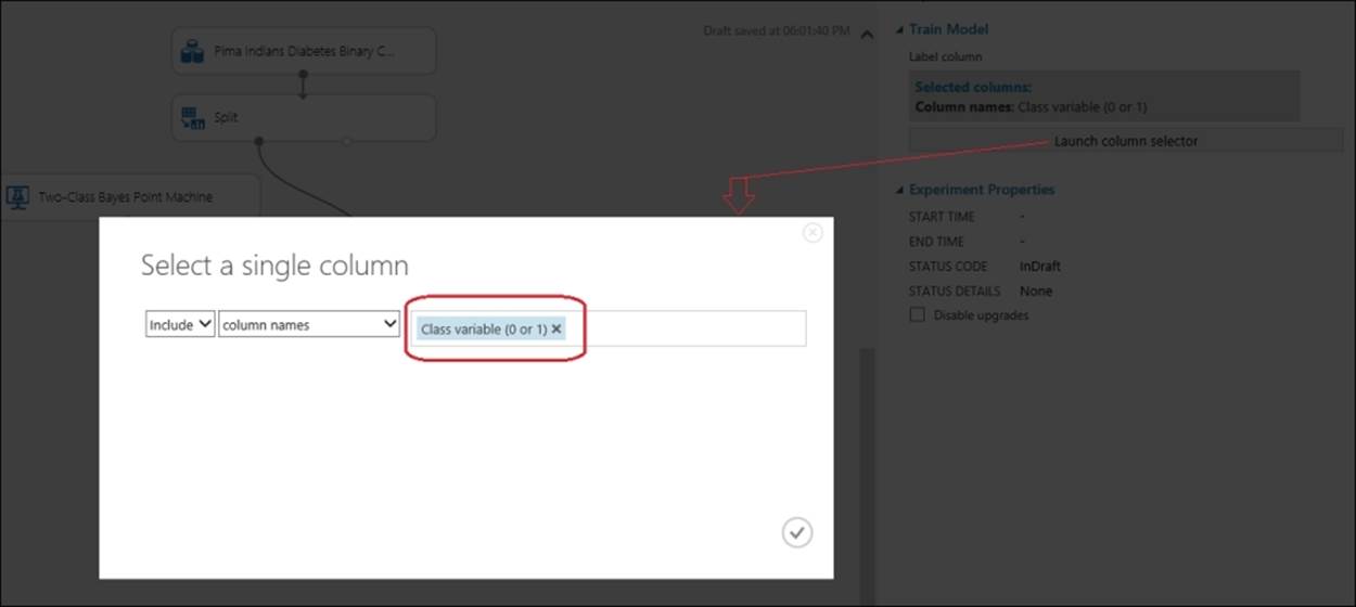
Drag the Train Model module to the canvas and connect the output port of the Two-Class Bayes Point Machine module to the first input port of the Train Model module. Connect the first output port of the Split module to the second input of the Train Model module. In the properties pane for the Train Model module, click on the Launch column selector button and when the pop-up appears, set Class variable (0 or 1) as the column's target variable, as shown in the following screenshot:

Next, drag the Score Model and Evaluate Model modules to the canvas. Connect the output of the Train Model module to the first input of the Score Model module and the second output of the Split module to the second input of the Score Model module. Then, connect the output of theScore Model module to the first input of the Evaluate Model module. Let's take a look at the following screenshot:

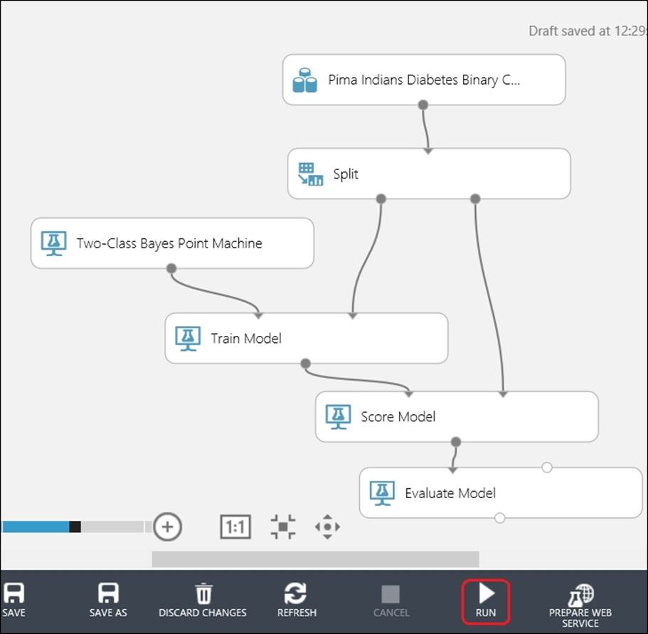
Click on RUN and run the experiment. When it finishes (after all the modules gets a green tick mark), right-click on the output of the Evaluate Model module and click on the Visualize option to view the Evaluation Results, as shown in the following screenshot:

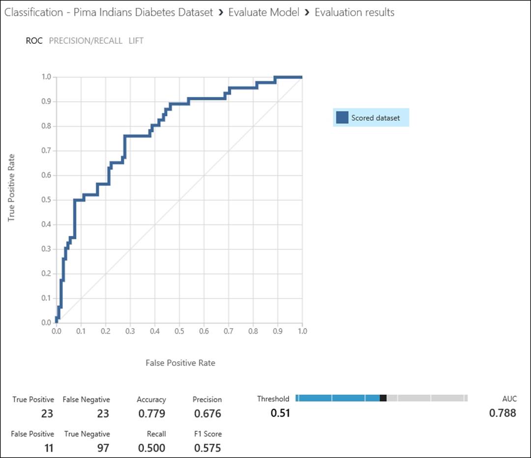
By default, the graph shows the ROC curve. The more area it covers, the better the model performs. This is represented by the matric AUC. AUC, as you can find here, is 0.788.

Note the Threshold scrollbar, which is set to 0.51 at the moment, which is 0.5 by default. You can increase or decrease it by dragging it to the left or right. As you change the value of threshold, all the other metrics apart from AUC get changed. The reason is obvious because when there are changes to the value of true positive and true negative, the rest of the values change. At the current value, the Threshold (0.51) Accuracy option is set at 77.9 percent.

You can also view the graph for precision/recall and lift by clicking on the respective tab at the top-left corner of the screen.

Two-class neural network with parameter sweeping

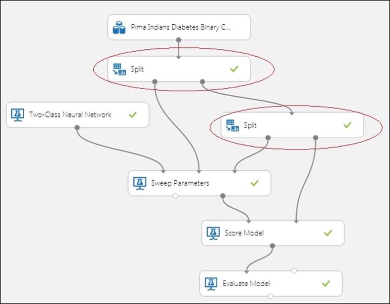
We will use the same diabetes dataset that we used to build the model using the neural network and to tune the parameter by parameter sweeping.

Create a new experiment. Drag and connect the same dataset to the Split module, as you did in the previous section. Set 0.8 as the parameter; Fraction of rows in the first output dataset is split into 80-20 to get your train and test dataset, respectively.

Type Sweep in the search box in the modules palette to the left of the screen and when the Sweep Parameters module appears, drag it to the canvas. Then, join the first output of the Split module to the second input of the Sweep Parameters module and join the second output of the Splitmodule to the third input of the Sweep Parameters module. Let's take a look at the following screenshot:

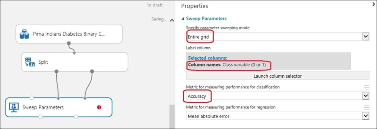
Now, you need to set the column of the dataset that is your target or label or class column for which you will train a model to make a prediction. In this case, Class variable (0 or 1) is the target variable or class for which you are going to make a prediction. Also, set the sweeping mode toEntire grid and Metric for measure the performance for Classification to Accuracy. Ignore the other parameter as this is a classification problem.

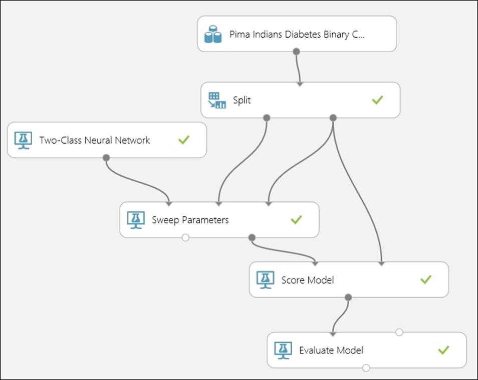
Type Two-Class Neural Network in search box at the top of the modules palette to the left and drag the Two-Class Neural Network module to the canvas. Connect it to the first input of the Sweep Parameters module. As usual, drag the Score Model and Evaluate Model modules to the canvas and make the necessary connections.

Connect the second output port of the Sweep Parameters module to the first input port of the Score Model module and connect the second output of the Split module to the second input of the Score Model module. Then, connect the output of the Score Model module to the first input of the Evaluate Model module.

Run the experiment. Let's take a look at the following screenshot:

As the experiment finishes running, visualize the output of the Evaluate Model module to measure the performance of the model. Note the AUC and accuracy metrics.

While using parameter sweeping to find the best parameters for the model, it is a good practice to use a separate dataset to score and evaluate the prediction than what is used for training and parameter tuning. To illustrate the point, you can split your dataset into 60 percent and 40 percent. Then, use another split module to split the 40 percent (the second dataset) into 50 percent each. So now, you have three datasets containing 60 percent, 20 percent, and 20 percent of your original dataset. Then, use the first 60 percent and 20 percent for the Sweep Parameters module and the rest 20 percent for scoring and evaluation. Let's take a look at the following screenshot:

Predicting adult income with decision-tree-based models

ML Studio comes with three decision-tree-based algorithms for two-class classification: the Two-Class Decision Forest, Two-Class Boosted Decision Tree, and Two-Class Decision Jungle modules. These are known as ensemble models where more than one decision trees are assembled to obtain better predictive performance. Though all the three are based on decision trees, their underlying algorithms differ.

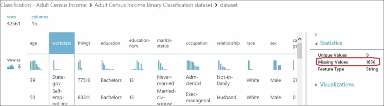
We will first build a model with the Two-Class Decision Forest module and then compare it with the Two-Class Boosted Decision Tree module for the Adult Census Income Binary Classification dataset module, which is one of the sample datasets available in ML Studio. The dataset is a subset of the 1994 US census database and contains the demographic information of working adults over the 16 years age limit. Each instance or example in the dataset has a label or class variable that states whether a person earns 50K a year or not.

Create an experiment and drag the dataset from the Saved Datasets group in the module palette. Right-click on the output port and click on Visualize to explore the dataset. When you click on the different columns, you can find that these columns contain a large number of missing values:workclass, occupation, and native-country. Other columns don't have missing values. Let's take a look at the following screenshot:

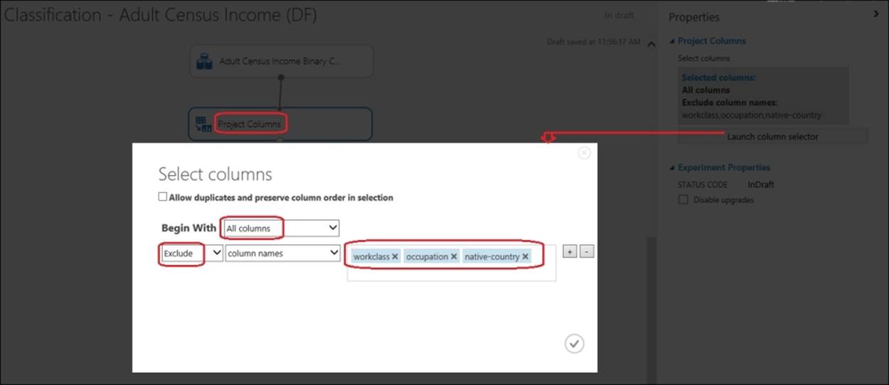
Though it would still work, if you still build models with missing values, we would get rid of these columns in our models. Missing values may impact the predicted result.

In the search box, type Project and drag the Project Columns module to the canvas. Connect the dataset module to this module. On the properties pane, click on the Launch Column Selector module, so that the pop-up columns selector comes up. As you can see in the following screenshot, begin with all the columns and exclude the columns with the missing values: workclass, occupation, and native-country:

Expand the Data Transformation group and then expand the Sample and Split option in the modules palette and drag the Split module to the canvas. Set the Fraction of rows parameter in the first output dataset to 0.8 and leave the others at their default values. You are splitting the dataset so that 80 percent of the data will be used to train and rest 20 percent will be used for test.

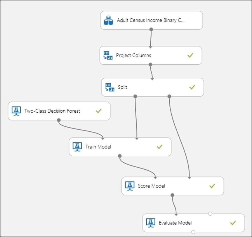
Likewise, now drag the Two-Class Decision Forest module to the canvas. Type Decision Forest in the search box in the modules palette to the left and when the module appears, drag it to the canvas. Set the Resampling method property to Bagging and leave the rest of the parameters at their default values. Leave the module with the default values for the properties.

Drag a Train Model module to the canvas and connect the output port of the Two-Class Decision Forest module to the first input port of the Train Model module. Connect the first output port of the Split module to the second input of the Train Model module. In the properties pane for the Train module, click on the column selector option and set income as the column's target variable.

Next, drag the Score Model and Evaluate Model modules to the canvas. Connect the output of the Train Model module to the first input of the Score Model module and connect the second output of the Split module to the second input of the Score Model module. Then, connect the output of the Score Model module to the first input of the Evaluate Model module.

Run the experiment and after its successful execution, visualize the evaluation result. Let's take a look at the following screenshot:

As with any experiment, you can now compare your model with another algorithm. You built a model using the Two-Class Decision Forest module. Now, use another algorithm, such as the Two-Class Boosted Decision Tree module and evaluate it.

To do so, start with the experiment and select the Train and Score modules by pressing ctrl on your keyboard and clicking on both the modules. Then, copy the selected modules and paste them on the canvas by right-clicking on them and pasting them or just by pressing ctrl + v on your keyboard. It supports copy paste much like any other MS product, for example, MS Word.

Now, click anywhere on the canvas to unselect the pasted modules and rearrange them so that no module is placed on another and all are readable. Remove the connection between the Two-Class Decision Forest and the Train Model modules by selecting them and pressing Delete. Drag theTwo-Class Boosted Decision Tree module from the left-hand side palette, to the canvas and connect the output of the module to the Train Model module. Leave it at the default property values. Connect the output of the Score Model module to the second input of the Evaluate Modelmodule and run the experiment. Let's take a look at the following screenshot:

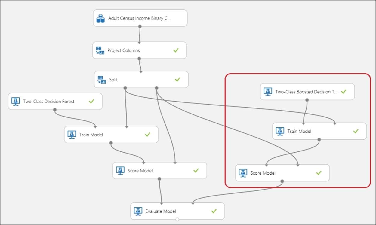
After the successful run, right-click on the output port of the Evaluate Model module and click on Visualize to find the evaluation result of the two models on a single canvas.

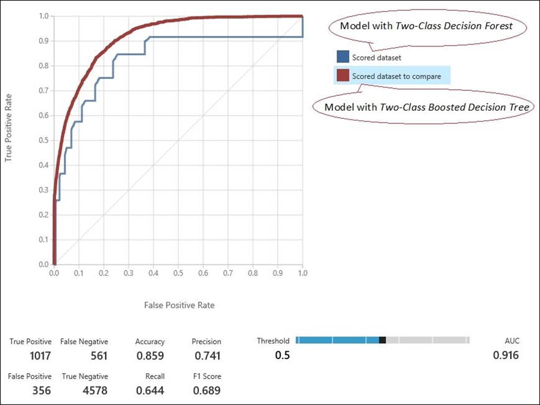
As you can see in the preceding graph, with the current settings, the model with the Two-Class Boosted Decision Tree module has higher values than the other when you see the AUC and accuracy figures.

So, we know that it is performing better than the other one.

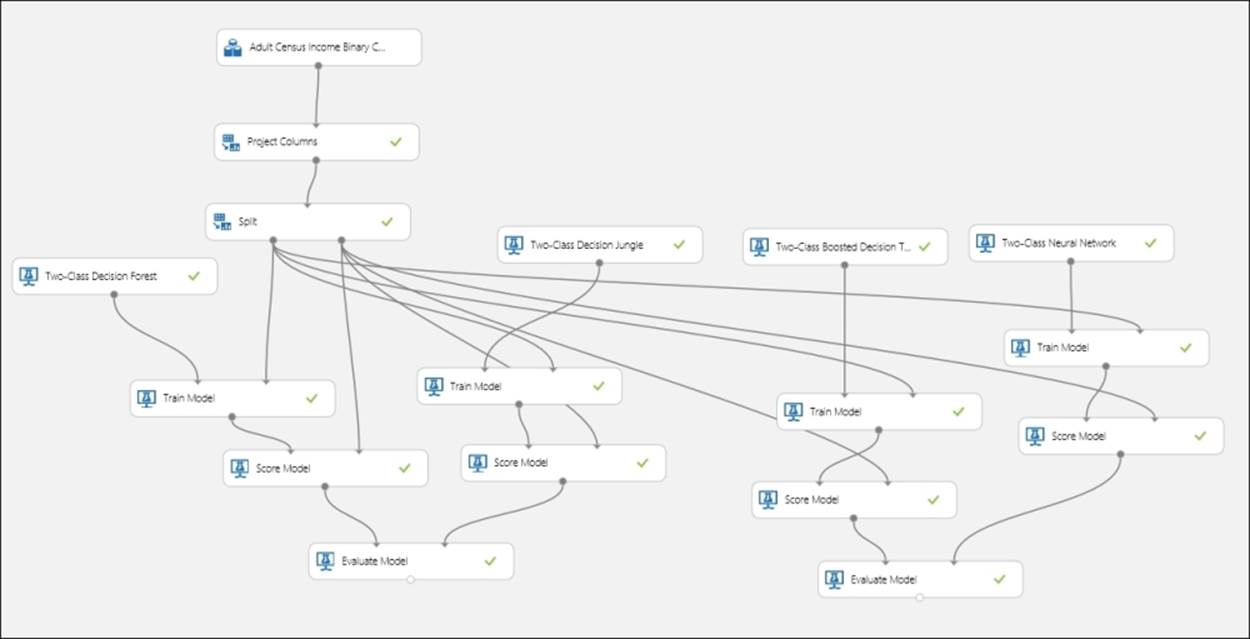
Do it yourself – comparing models to choose the best

You have already tried two algorithms for the Adult Census Income Binary Classification dataset module. Now, try another two modules to choose the best one for your final model: the Two-Class Boosted Decision Tree and the Two-Class Neural Network modules. Try out different parameters; use the Sweep Parameters module to optimize the parameters for the algorithms. The following screenshot is just for your reference—your experiment might differ. You may also try this with other available algorithms, for example, the Two-Class Averaged Perceptron or theTwo-Class Logistic Regression modules to find the best model. Let's take a look at the following screenshot:

Multiclass classification

The classification you have seen and experienced so far is a two-class classification where the target variable can be of two classes. In multiclass classification, you classify in more than two classes, for example continuing on our hypothetical tumor problem, for a given tumor size and age of a patient, you might predict one of these three classes as the possibility of a patient being affected with cancer: High, Medium, and Low. In theory, a target variable can have any number of classes.

Evaluation metrics – multiclass classification

ML Studio lets you evaluate your model with an accuracy that is calculated as a ratio of the number of correct predictions versus the incorrect ones. Consider the following table:

The following can be the evaluation metrics where in the columns, the text is marked in bold and have background colors according to the accuracy per class. For example, there were three actual classes as Medium, but only two were correctly predicted, so accuracy = 2/ 3 = 66.6 %. It also shows that 33.3 percent of the Medium class was inaccurately predicted as High. This is also known as the confusion matrix. Let's take a look at the following table:

Multiclass classification with the Iris dataset

The Iris dataset is one of the classic and simple datasets. It contains the observations about the Iris plant. Each instance has four features: the sepal length, sepal width, petal length, and petal width. All the measurements are in centimeters. The dataset contains three classes for the target variable, where each class refers to a type of Iris plant: Iris Setosa, Iris Versicolour, and Iris Virginica.

You can find more information on this dataset at http://archive.ics.uci.edu/ml/datasets/Iris.

As this dataset is not present as a sample dataset in ML Studio, you need to import it to ML Studio using a reader module before building any model on it. Note that the Iris dataset present in the Saved Dataset section is the subset of the original dataset and is only present for two classes.

Multiclass decision forest

Decision forest is also available for multiclass classification. We will first use this with parameter sweep to train the model.

Follow the given steps to import the Iris dataset:

1. Go to ML Studio. Click on the +NEW button and choose Blank Experiment.

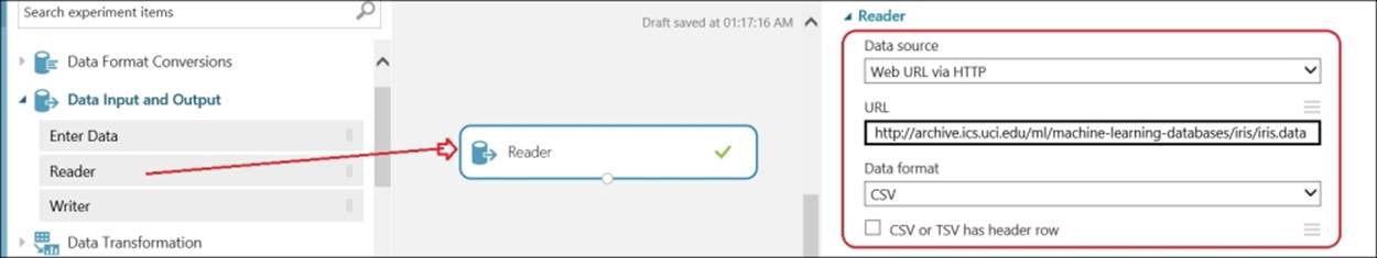
2. From the modules palette, find the Reader module under the Data Input and Output group and drag it to the experiment canvas.

3. The module properties pane is displayed after this. Choose the data source as HTTP.

4. Specify a complete URL: http://archive.ics.uci.edu/ml/machine-learning-databases/iris/iris.data.

5. Specify the data format as CSV.

6. Don't tick the checkbox for the header row, as the dataset does not contain any header. You might end up with something as follows:

Run the experiment and when you see the green tick mark on the Reader module, right-click on the output port and click on Visualize. Clicking on any column, you can notice that ML Studio shows a missing value.

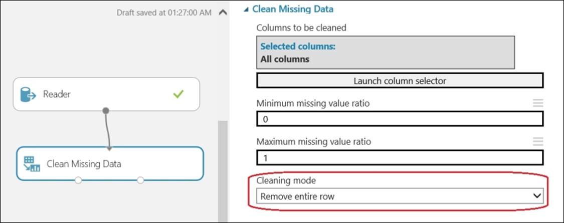
Use the Clean Missing Data module to remove the row containing the missing value. Drag the module that can be found under the Data Transformation group and then under Manipulation in the modules palette to the canvas. Connect the output port of the Reader module to the input port of this module. On the properties pane, choose Remove entire row for the property for Cleaning mode, as shown in the following screenshot:

Expand the Data Transformation group and then expand the Sample and Split option in the modules palette and drag the Split module to the canvas. Set the Fraction of rows parameter in the first output dataset to 0.7 and leave the others at their default values. You are splitting the dataset so that 70 percent of the data will be used to train and the other 30 percent will be used for test.

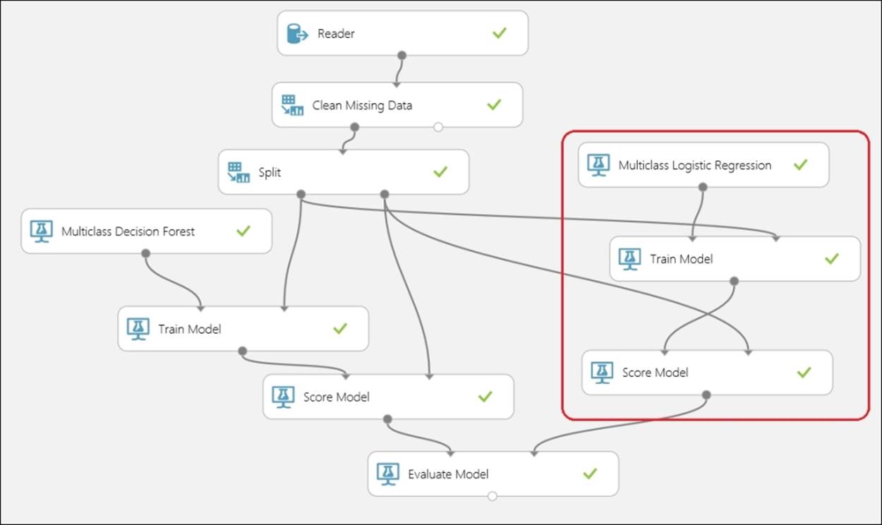
Likewise, now drag the Multiclass Decision Forest module to canvas. To do so, type Decision Forest in the search box in the modules palette to the left and when the module appears, drag it to the canvas. Set the Resampling method property to Bagging and leave the rest of the properties at their default values. Leave the module with the default values for the properties.

Drag a Train Model module to the canvas and connect the output port of the Multiclass Decision Forest module to the first input port of the Train Model module. Connect the first output port of the Split module to the second input of the Train Medel module. In the properties pane for theTrain Model module, click on the column selector and set Col5 as the column's target variable.

Next, drag the Score Model and Evaluate Model modules to the canvas. Connect the output of the Train Model module to the first input of the Score Model module and connect the second output of the Split module to the second input of the Score Model module. Then, connect the output of the Score Model module to the first input of the Evaluate Model module. Let's take a look at the following screenshot:

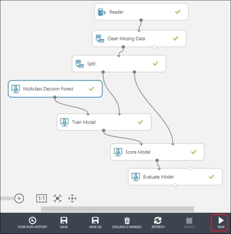
Now, run the experiment and after its completion, visualize the output of the Evaluate Model module to know the performance of the model.

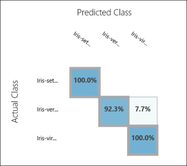
As you can see in the preceding graph, the Iris Versicolour class has 92.3% accuracy, while others have 100%. Also, 7.7% of the time the Iris Versicolour class has been misclassified as Iris Virginica.

Note that you have not done any optimization by tuning the parameters. You can try out different values for the parameters and evaluate the performance or simply use the Sweep Parameters module to get the best parameters.

Comparing models – multiclass decision forest and logistic regression

As with any experiment, you can now compare your model with another algorithm. You built a model using multiclass decision forest. Now, use another algorithm, such as multiclass logistic regression to evaluate the prediction.

To do so, start with the experiment and select the Train and Score modules by pressing ctrl on your keyboard and click on both the modules. Then, copy the selected modules and paste them on the canvas by right-clicking on it and pasting them or just by pressing ctrl + v on your keyboard. Now, click anywhere on the canvas to unselect the pasted modules and rearrange them so that no module is placed on another and all are readable. Let's take a look at the following screenshot:

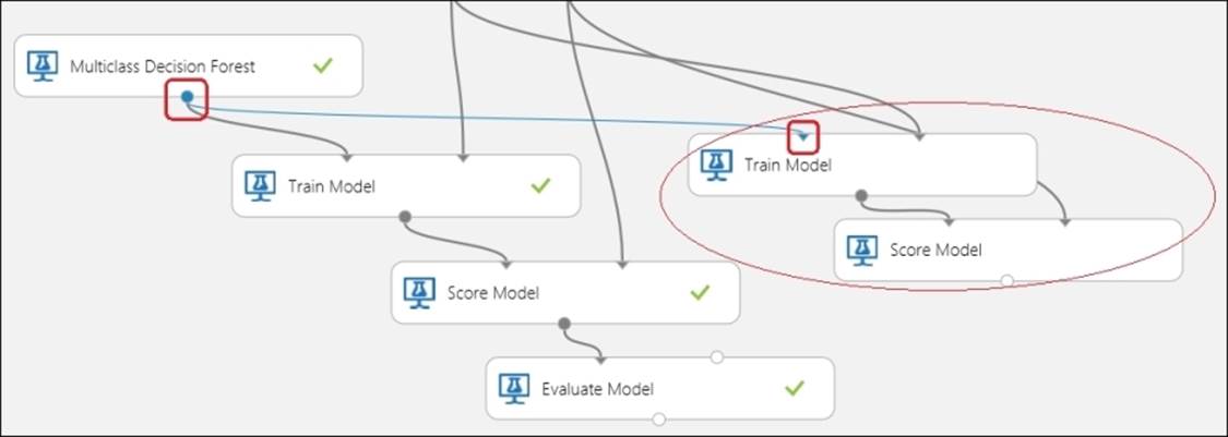
Now, remove the connection between the Multiclass Decision Forest and Train Model modules by selecting the connection and pressing Delete. Note the connection in the preceding screenshot. Drag the Multiclass Logistic Regression module from the left-hand side palette to the canvas and connect the output of the module to the Train Model module. Leave the properties of the Multiclass Logistic Regression module at their default values. Connect the output of the Score Model module to the second input of the Evaluate Model module. Let's take a look at the following screenshot:

You can run the model to find out how the new model is performing and then you can compare the evaluation metrics. After the experiment finishes running, visualize the output of the Evaluate Model module to know the performance of the model.

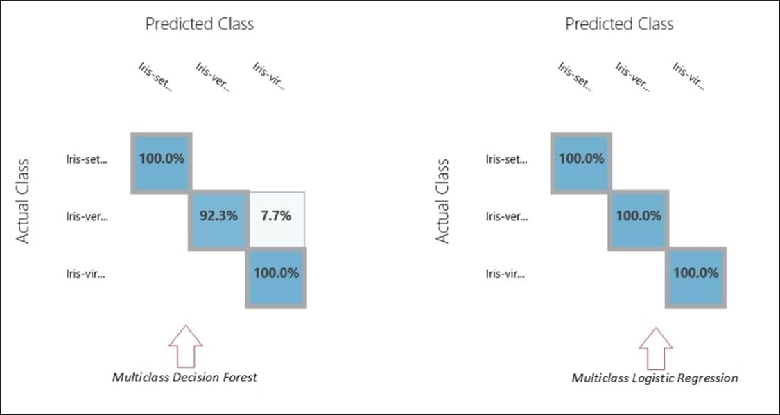
As you can note, for the model with the logistic regression, you are getting 100% accuracy for all the classes. Given such a scenario, you know which model to pick up.

Multiclass classification with the Wine dataset

The Wine dataset is another classic and simple dataset hosted in the UCI machine learning repository. It contains chemical analysis of the content of wines grown in the same region in Italy, but derived from three different cultivars. It is used to determine models for classification problems by predicting the source (cultivar) of wine as class or target variable. The dataset has the following 13 features (dependent variables), which are all numeric:

· Alcohol

· Malic acid

· Ash

· Alcalinity of ash

· Magnesium

· Total phenols

· Flavanoids

· Nonflavanoid phenols

· Proanthocyanins

· Color intensity

· Hue

· OD280/OD315 of diluted wines

· Proline

The examples or instances are classified into three classes: 1, 2 and 3.

You can find more about the dataset at http://archive.ics.uci.edu/ml/datasets/Wine.

Multiclass neural network with parameter sweep

We will build a model with multiclass neural network and optimize the parameters with the Sweep Parameter module.

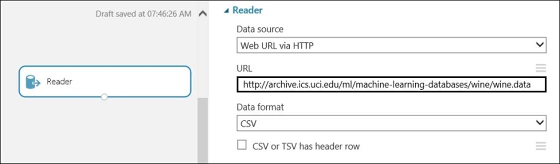
As you did the last time, use the Reader module to import the dataset from http://archive.ics.uci.edu/ml/machine-learning-databases/wine/wine.data.

It is in the CSV format and has no header row, as shown in the following screenshot:

Use the Split module and split it into the ratio of 70:30 for a train and test dataset, respectively.

Type Sweep in the search box in the modules palette to the left and when the Sweep Parameters module appears, drag it to the canvas. Then, join the first output of the Split module to the second input of the Sweep Parameters module and join the second output of the Split module to the third input of the Sweep Parameters module.

Now, you need to set the column of the dataset that is your target, label, or class column for which you will train a model to make a prediction. In this case, Col1 is the target variable or class for which you are going to make a prediction. Also, set the sweeping mode to Entire grid for metric to measure the performance of the Classification to Accuracy option.

Also, get the Multiclass Neural Network module and connect it to the first input of the Sweep Parameters module. As usual, drag the Score Model and Evaluate Model modules to the canvas. Connect the second output port of the Sweep Parameters module to the first input port of theScore Model module and connect the second output of the Split module to the second input of the Score Model module. Then, connect the output of the Score Model module to the first input of the Evaluate Model module.

Run the experiment.

As the experiment finishes running, visualize the output of the Evaluate Model module to know the performance of the model.

Do it yourself – multiclass decision jungle

Use the same Wine dataset and build a model using the Multiclass Decision Jungle module. You can use the Sweep Parameters module to optimize the parameters of the algorithms. After you run the experiment, check out the evaluation metrics. Do you find any improvement in the performance than the previous model you built with neural network or any other available algorithms?

Summary

You started the chapter with understanding predictive analysis with classification and explored the concepts of training, testing, and validating a classification model. You then proceeded to carry on building experiments with different two-class and multiclass classification models, such as logistic regression, decision forest, neural network, and boosted decision trees inside ML Studio. You learned how to score and evaluate a model after training. You also learned how to optimize different parameters for a learning algorithm by the module, Sweep Parameters.

After exploring the two-class classification, you understood multiclass classification and learnt how to evaluate a model for the same. You then built a couple of models for multiclass classification using different available algorithms.

In the next chapter, you will explore the process of building a model using clustering, an unsupervised learning algorithm.