Excel Data Analysis For Dummies, 2nd Edition (2014)
Part III. Advanced Tools
 Visit www.dummies.com/extras/exceldataanalysis for more on how to improve your Excel formula-building skills.
In this part …
· Use database statistical functions to analyze selected information in a table or list.
· Tap into the power of Excel’s more than 70 statistical functions to calculate averages, determine ranking and percentiles, measure dispersions, and analyze distributions.
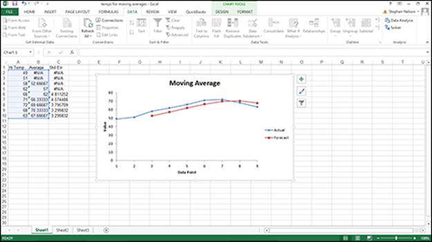
· Gain extra insights into your data by using the Data Analysis add-on tool for creating histograms, calculating moving averages, using exponential smoothing, and performing smart sampling.
· Use the regression and correlation tools, the ANOVA data analysis tool, and the z-test, t-test, and Fourier data analysis tools to perform inferential statistics analysis.
Chapter 8. Using the Database Functions
In This Chapter
![]() Reviewing function basics
Reviewing function basics
![]() Using the DAVERAGE function
Using the DAVERAGE function
![]() Using the DCOUNT and DCOUNTA functions
Using the DCOUNT and DCOUNTA functions
![]() Using the DGET function
Using the DGET function
![]() Using the DMAX and DMIN functions
Using the DMAX and DMIN functions
![]() Using the DPRODUCT function
Using the DPRODUCT function
![]() Using the DSTDEV and DSTDEVP functions
Using the DSTDEV and DSTDEVP functions
![]() Using the DSUM function
Using the DSUM function
![]() Using the DVAR and DVARP functions
Using the DVAR and DVARP functions
Excel provides a special set of functions, called database functions, especially for simple statistical analysis of information that you store in Excel tables. In this chapter, I describe and illustrate these functions.
 Are you interested in statistical analysis of information that’s not stored in an Excel table? Then you can use this chapter as a resource for descriptions of functions that you use for analysis when your information isn’t in an Excel table.
Note: Excel also provides a rich set of statistical functions, which are also wonderful tools for analyzing information in an Excel table. Skip to Chapter 9 for details on these statistical functions.
Quickly Reviewing Functions
The Excel database functions work like other Excel functions. In a nutshell, when you want to use a function, you create a formula that includes the function. Because I don’t discuss functions in detail anywhere else in this book — and because you need to be relatively proficient with the basics of using functions in order to employ them in any data analysis — I review some basics here, including function syntax and entering functions.
Understanding function syntax rules
Most functions need arguments, or inputs. In particular, all database functions need arguments. You include these arguments inside parentheses. If a function needs more than one argument, you can separate arguments by using commas.
For illustration purposes, here are a couple of example formulas that use simple functions. These aren’t database functions, by the way. I get to those in later sections of this chapter. Read through these examples to become proficient with the everyday functions. (Or just breeze through these as a refresher.)
You use the SUM function to sum, or add up, the values that you include as the function arguments. In the following example, these arguments are 2, 2, the value in cell A1, and the values stored in the worksheet range B3:G5.
=SUM(2,2,A1,B3:G5)
Here’s another example. The following AVERAGE function calculates the average, or arithmetic mean, of the values stored in the worksheet range B2:B100.
=AVERAGE(B2:B100)
Simply, that’s what functions do. They take your inputs and perform some calculation, such as a simple sum or a slightly more complicated average.
Entering a function manually
How you enter a function-based formula into a cell depends on whether you’re familiar with how the function works — at least roughly.
If you’re familiar with how a function works — or at the very least, you know its name — you can simply type an equals sign followed by the function name into the cell. SUM and AVERAGE are good examples of easy-to-remember function names. When you type that first parenthesis [(] after entering the full function name, Excel displays a pop-up ScreenTip that names the function arguments and shows their correct order. (Refer to the previous section, “Understanding function syntax rules,” if you need to brush up on some mechanics.) In Figure 8-1, for example, you can see how this looks in the case of the loan payment function, which is named PMT.
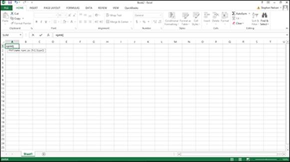
Figure 8-1: The ScreenTip for the PMT function identifies function arguments and shows their correct order.
If you point to the function name in the ScreenTip, Excel turns the function name into a hyperlink. Click the hyperlink to open the Excel Help file and see its description and discussion of the function.
Entering a function with the Function command
If you’re not familiar with how a function works — maybe you’re not even sure what function that you want to use — you need to use the Formulas tab’s Insert Function command to find the function and then correctly identify the arguments.
To use the Function Wizard command in this manner, follow these steps:
1. Position the cell selector at the cell into which you want to place the function formula.
You do this in the usual way. For example, you can click the cell. Or you can use the navigation keys, such as the arrow keys, to move the cell selector to the cell.
2. Choose the Formulas tab’s Function Wizard command.
Excel displays the Insert Function dialog box, as shown in Figure 8-2.
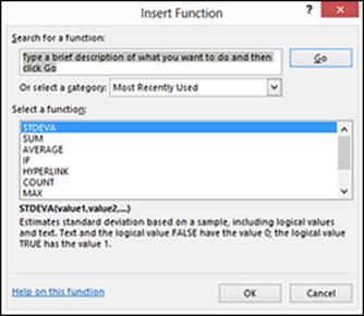
Figure 8-2: Select a function here.
3. In the Search for a Function text box, type a brief description of what you want to calculate by using a function.
For example, if you want to calculate a standard deviation for a sample, type something like standard deviation.
4. Click the Go button.
In the Select a Function list box, Excel displays a list of the functions that might just work for you, as shown in Figure 8-3.
Note: The STDEVPA function in Figure 8-3 isn’t a database function, so I don’t describe it in this chapter. Read through Chapter 9 for more on this function.
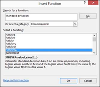
Figure 8-3: Let Excel help you narrow down the function choices.
5. Find the right function.
To find the right function for your purposes, first select a function in the Select a Function list. Then read the full description of the function, which appears beneath the function list. If the function you select isn’t the one you want, select another function and read its description. Repeat this process until you find the right function.
If you get to the end of the list of functions and still haven’t found what you want, consider repeating Step 3, but this time use a different (and hopefully better) description of the calculation you want to make.
6. After you find the function you want, select it and then click OK.
Excel displays the Function Arguments dialog box, as shown in Figure 8-4.
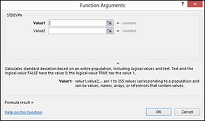
Figure 8-4: Supply function arguments here.
7. Supply the arguments.
To supply the arguments that a function needs, click an argument text box (Value1 and Value2 in Figure 8-4). Next, read the argument description, which appears at the bottom of the dialog box. Then supply the argument by entering a value, formula, or cell or range reference into the argument text box.
If a function needs more than one argument, repeat this step for each argument.
Excel calculates the function result based on the arguments that you enter and displays this value at the bottom of the dialog box next to Formula Result =, as shown in Figure 8-5.
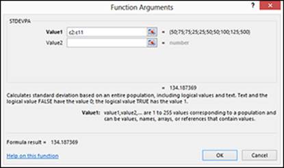
Figure 8-5: Enter arguments, and Excel calculates them for you.
8. (Optional) If you need help with a particular function, browse the Excel Help information.
If you need help using some function, your first resource — yes, even before you check this chapter — should be to click the Help on This Function hyperlink, which appears in the bottom-left corner of the Function Arguments dialog box. In Figure 8-6, you can see the help information that Excel displays for the STDEVPA function.
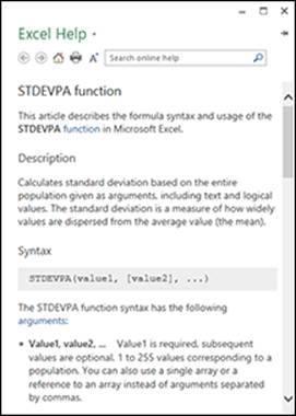
Figure 8-6: Ask Excel for function help.
9. When you’re satisfied with the arguments that you enter in the Function Arguments dialog box, click OK.
And now it’s party time. In the next section, I describe each of the database statistical functions that Excel provides.
The Or Select a Category drop-down list
After you learn your way around Excel and develop some familiarity with its functions, you can also narrow down the list of functions by selecting a function category from the Or Select a Category drop-down list in the Insert Function dialog box. For example, if you select Database from this drop-down list, Excel displays a list of its database functions. In some cases, this category-based approach works pretty darn well. It all depends, really, on how many functions Excel puts into a category. Excel provides 12 database functions, so that’s a pretty small set. Other sets, however, are much larger. For example, Excel supplies more than 70 statistical functions. For large categories, such as the statistical functions category, the approach that I suggest in the section “Entering a function with the Function command” (see Step 3 there) usually works best.
Using the DAVERAGE Function
The DAVERAGE function calculates an average for values in an Excel list. The unique and truly useful feature of DAVERAGE is that you can specify that you want only list records that meet specified criteria included in your average.
If you want to calculate a simple average, use the AVERAGE function. In Chapter 9, I describe and illustrate the AVERAGE function.
The DAVERAGE function uses the following syntax:
=DAVERAGE(database,field,criteria)
where database is a range reference to the Excel table that holds the value you want to average, field tells Excel which column in the database to average, and criteria is a range reference that identifies the fields and values used to define your selection. The field argument can be a cell reference holding the field name, the field name enclosed in quotation marks, or a number that identifies the column (1 for the first column, 2 for the second column, and so on).
As an example of how the DAVERAGE function works, suppose that you’ve constructed the worksheet shown in Figure 8-7. Notice that the worksheet range holds a small table. Row 1 predictably stores field names: Name, State, and Donation. Rows 2–11 store individual records.

Figure 8-7: Use the DAVERAGE database statistical functions to calculate an average for values in an Excel table.
If you’re a little vague on what an Excel table (or list) is, you should take a peek at Chapter 1. Excel database functions analyze information from Excel tables, so you need to know how tables work in order to easily use database functions.
Rows 14 and 15 store the criteria range. The criteria range typically duplicates the row of field names. The criteria range also includes at least one other row of labels or values or Boolean logic expressions that the DAVERAGE function uses to select records from the list. In Figure 8-7, for example, note the Boolean expression in cell C15, <500, which tells the function to include only records where the Donation field shows a value less than 500.
The DAVERAGE function, which appears in cell F3, is
=DAVERAGE(A1:C11,"Donation",A14:C15)
and it returns the average donation amount shown in the database list, excluding the donation from Jeannie in California because that amount isn’t less than 500. The actual function result is 63.88889.
Although I mention this in a couple of other places in this book, I want to repeat something important: Each row in your criteria range is used to select records for the function. For example, if you use the criteria range shown in Figure 8-8, you select records using two criteria. The criterion in row 15 tells the DAVERAGE function to select records where the donation is less than 500. The criterion in row 16 tells the DAVERAGE function to select records where the state is California. The DAVERAGE function, then, uses every record in the list because every record meets at least one of the criteria. The records in the list don't have to meet both criteria; just one of them.

Figure 8-8: Using a criteria range that’s a little more complicated.
To combine criteria — suppose that you want to calculate the DAVERAGE for donations from California that are less than 500 — you put both the criteria into the same row, as shown in row 15 of Figure 8-9.
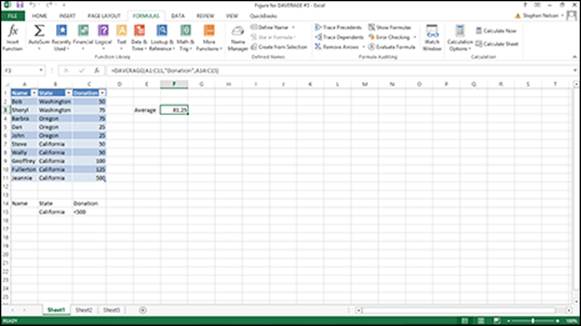
Figure 8-9: You can combine the criteria in a range.
Using the DCOUNT and DCOUNTA Functions
The DCOUNT and DCOUNTA functions count records in a database table that match criteria that you specify. Both functions use the same syntax, as shown here:
=DCOUNT(database,field,criteria)
=DCOUNTA(database,field,criteria)
where database is a range reference to the Excel table that holds the value that you want to count, field tells Excel which column in the database to count, and criteria is a range reference that identifies the fields and values used to define your selection criteria. The fieldargument can be a cell reference holding the field name, the field name enclosed in quotation marks, or a number that identifies the column (1 for the first column, 2 for the second column, and so on).
Excel provides several other functions for counting cells with values or labels: COUNT, COUNTA, COUNTIF, and COUNTBLANK. Refer to Chapter 9 or the Excel online help for more information about these tools.
The functions differ subtly, however. DCOUNT counts fields with values; DCOUNTA counts fields that aren’t empty.
As an example of how the DCOUNT and DCOUNTA functions work, suppose that you’ve constructed the worksheet shown in Figure 8-10, which contains a list of players on a softball team. Row 1 stores field names: Player, Age, and Batting Average. Rows 2–11 store individual records.
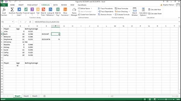
Figure 8-10: Use the DCOUNT and DCOUNTA database statistical functions to count records in a database list.
Rows 14 and 15 store the criteria range. Field names go into the first row. Subsequent rows provide labels or values or Boolean logic expressions that the DCOUNT and DCOUNTA functions use to select records from the list for counting. In Figure 8-10, for example, there’s a Boolean expression in cell B15, >8, which tells the function to include only records where the Age shows a value greater than eight. In this case, then, the functions count players on the team who are older than 8.
The DCOUNT function, which appears in cell F3, is
=DCOUNT(A1:C11,C1,A14:C15)
The function counts the players on the team who are older than 8. But because the DCOUNT function looks only at players with a batting average in the Batting Average field, it returns 8. Another way to say this same thing is that in this example, DCOUNT counts the number of players on the team who are older than 8 and have a batting average.
If you want to get fancy about using Boolean expression to create your selection criteria, take a peek at the earlier discussion of the DAVERAGE function. In that section, “Using the DAVERAGE Function,” I describe how to create compound selection criteria.
The DCOUNTA function, which appears in cell F5, is
=DCOUNTA(A1:C11,3,A14:C15)
The function counts the players on the team who are older than 8 and have some piece of information entered into the Batting Average field. The function returns the value 9 because each of the players older than 8 have something stored in the Batting Average field. Eight of them, in fact, have batting average values. The fifth player (Christina) has the text label NA.
If you just want to count records in a list, you can omit the field argument from the DCOUNT and DCOUNTA functions. When you do this, the function just counts the records in the list that match your criteria without regard to whether some field stores a value or is nonblank. For example, both of the following functions return the value 9:
=DCOUNT(A1:C11,A14:C15)
=DCOUNTA(A1:C11,A14:C15)
Note: To omit an argument, you just leave the space between the two commas empty.
Using the DGET Function
The DGET function retrieves a value from a database list according to selection criteria. The function uses the following syntax:
=DGET(database,field,criteria)
where database is a range reference to the Excel table that holds the value you want to extract, field tells Excel which column in the database to extract, and criteria is a range reference that identifies the fields and values used to define your selection criteria. The fieldargument can be a cell reference holding the field name, the field name enclosed in quotation marks, or a number that identifies the column (1 for the first column, 2 for the second column, and so on).
Go back to the softball players list example in the preceding section. Suppose that you want to find the batting average of the single eight-year-old player. To retrieve this information from the list shown in Figure 8-11, enter the following formula into cell F3:
=DGET(A1:C11,3,A14:C15)
This function returns the value 0.444 because that’s the eight-year-old’s batting average.
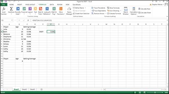
Figure 8-11: Use DGET to retrieve a value from a database list based on selection criteria.
By the way, if no record in your list matches your selection criteria, DGET returns the #VALUE error message. For example, if you construct selection criteria that look for a 12-year-old on the team, DGET returns #VALUE because there aren’t any 12-year-old players. Also, if multiple records in your list match your selection criteria, DGET returns the #NUM error message. For example, if you construct selection criteria that look for a ten-year-old, DGET returns the #NUM error message because four ten-year-olds are on the team.
Using the DMAX and DMAX Functions
The DMAX and DMIN functions find the largest and smallest values, respectively, in a database list field that match the criteria that you specify. Both functions use the same syntax, as shown here:
=DMAX(database,field,criteria)
=DMIN(database,field,criteria)
where database is a range reference to the Excel table, field tells Excel which column in the database to look in for the largest or smallest value, and criteria is a range reference that identifies the fields and values used to define your selection criteria. The field argument can be a cell reference holding the field name, the field name enclosed in quotation marks, or a number that identifies the column (1 for the first column, 2 for the second column, and so on).
Excel provides several other functions for finding the minimum or maximum value, including MAX, MAXA, MIN, and MINA. Turn to Chapter 9 for more information about using these related functions.
As an example of how the DMAX and DMIN functions work, suppose you construct a list of your friends and some important statistical information, including their typical golf scores and their favorite local courses, as shown in Figure 8-12. Row 1 stores field names: Friend, Golf Score, and Course. Rows 2–11 store individual records.
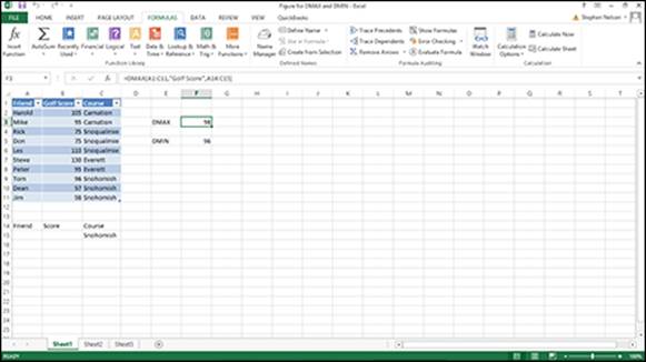
Figure 8-12: Use the DMAX and DMIN database statistical functions to find the largest and smallest values.
Rows 14 and 15 store the criteria range. Field names go into the first row. Subsequent rows provide labels or values or Boolean logic expressions that the DMAX and DMIN functions use to select records from the list for counting. In Figure 8-12, for example, note the text label in cell C15, Snohomish, which tells the function to include only records where the Course field shows the label Snohomish.
The DMAX function, which appears in cell F3, is
=DMAX(A1:C11,"Golf Score",A14:C15)
The function finds the highest golf score of the friends who favor the Snohomish course, which happens to be 98.
If you want to get fancy about using Boolean expression to create your selection criteria, take a peek at the earlier discussion of the DAVERAGE function. In that section, “Using the DAVERAGE Function,” I describe how to create compound selection criteria.
The DMIN function, which appears in cell F5, is
=DMIN(A1:C11,"Golf Score",A14:C15)
The function counts the lowest score of the friends who favor the Snohomish course, which happens to be 96.
Using the DPRODUCT Function
The DPRODUCT function is weird. And I’m not sure why you would ever use it. Oh sure, I understand what it does. The DPRODUCT function multiplies the values in fields from a database list based on selection criteria. I just can’t think of a general example about why you would want to do this.
The function uses the syntax
=DPRODUCT(database,field,criteria)
where database is a range reference to the Excel table that holds the value you want to multiply, field tells Excel which column in the database to extract, and criteria is a range reference that identifies the fields and values used to define your selection criteria. If you’ve been reading this chapter from the very start, join the sing-along: The field argument can be a cell reference holding the field name, the field name enclosed in quotation marks, or a number that identifies the column (1 for the first column, 2 for the second column, and so on).
I can’t construct a meaningful example of why you would use this function, so no worksheet example this time. Sorry.
Note: Just so you don’t waste time looking, the Excel Help file doesn’t provide a good example of the DPRODUCT function either.
Using the DSTDEV and DSTDEVP Functions
The DSTDEV and DSTDEVP functions calculate a standard deviation. DSTDEV calculates the standard deviation for a sample. DSTDEVP calculates the standard deviation for a population. As with other database statistical functions, the unique and truly useful feature of DSTDEV and DSTDEVP is that you can specify that you want only list records that meet the specified criteria you include in your calculations.
If you want to calculate standard deviations without first applying selection criteria, use one of the Excel non-database statistical functions such as STDEV, STDEVA, STDEVP, or STDEVPA. In Chapter 9, I describe and illustrate these other standard deviation functions.
The DSTDEV and DSTDEVP functions use the same syntax:
=DSTDEV(database,field,criteria)
=DSTDEVP(database,field,criteria)
where database is a range reference to the Excel table that holds the values for which you want to calculate a standard deviation, field tells Excel which column in the database to use in the calculations, and criteria is a range reference that identifies the fields and values used to define your selection criteria. The field argument can be a cell reference holding the field name, the field name enclosed in quotation marks, or a number that identifies the column (1 for the first column, 2 for the second column, and so on).
As an example of how the DSTDEV function works, suppose you construct the worksheet shown in Figure 8-13. (This is the same basic worksheet as shown in Figure 8-7, in case you’re wondering.)
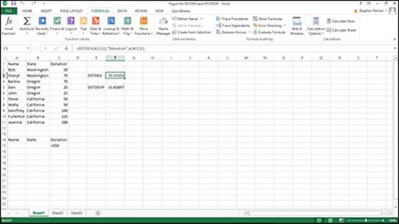
Figure 8-13: Calculate a standard deviation with the DSTDEV and DSTDEVP functions.
The worksheet range holds a small list with row 1 storing field names (Name, State, and Donation) and rows 2 through 11 storing individual records.
Rows 14 and 15 store the criteria range. The criteria range typically duplicates the row of field names. The criteria range also includes at least one other row of labels or values or Boolean logic expressions that the DSTDEV and DSTDEVP functions use to select records from the list. In Figure 8-13, for example, note the Boolean expression in cell C15, <250, which tells the function to include only records where the Donation field shows a value less than 250.
The DSTDEV function, which appears in cell F3, is
=DSTDEV(A1:C11,"Donation",A14:C15)
and it returns the sample standard deviation of the donation amounts shown in the database list, excluding the donation from Jeannie in California because that amount is not less than 250. The actual function result is 33.33333.
The DSTDEVP function, which appears in cell F5, is
=DSTDEVP(A1:C11,"Donation",A14:C15)
and returns the population standard deviation of the donation amounts shown in the database list excluding the donation from Jeannie in California because that amount isn’t less than 250. The actual function result is 31.42697.
You wouldn’t, by the way, simply pick one of the two database standard deviation functions willy-nilly. If you’re calculating a standard deviation using a sample, or subset of items, from the entire data set, or population, you use the DSTDEV function. If you’re calculating a standard deviation using all the items in the population, use the DSTDEVP function.
Using the DSUM Function
The DSUM function adds values from a database list based on selection criteria. The function uses the syntax:
=DSUM(database,field,criteria)
where database is a range reference to the Excel table, field tells Excel which column in the database to sum, and criteria is a range reference that identifies the fields and values used to define your selection criteria. The field argument can be a cell reference holding the field name, the field name enclosed in quotation marks, or a number that identifies the column (1 for the first column, 2 for the second column, and so on).
Figure 8-14 shows a simple bank account balances worksheet that illustrates how the DSUM function works. Suppose that you want to find the total of the balances that you have in open accounts paying more than 0.02, or 2 percent, interest. The criteria range in A14:D15 provides this information to the function. Note that both criteria appear in the same row. This means that a bank account must meet both criteria in order for its balance to be included in the DSUM calculation.
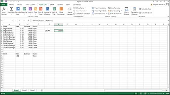
Figure 8-14: Add values from a database list with DSUM.
The DSUM formula appears in cell F3, as shown here:
=DSUM(A1:C11,3,A14:D15)
This function returns the value 39000 because that’s the sum of the balances in open accounts that pay more than 2 percent interest.
Using the DVAR and DVARP Functions
The DVAR and DVARP functions calculate a variance, which is another measure of dispersion — and actually, the square of the standard deviation. DVAR calculates the variance for a sample. DVARP calculates the variance for a population. As with other database statistical functions, using DVAR and DVARP enable you to specify that you want only those list records that meet selection criteria included in your calculations.
If you want to calculate variances without first applying selection criteria, use one of the Excel non-database statistical functions such as VAR, VARA, VARP, or VARPA. In Chapter 9, I describe and illustrate these other variance functions.
The DVAR and DVARP functions use the same syntax:
=DVAR(database,field,criteria)
=DVARP(database,field,criteria)
where database is a range reference to the Excel table that holds the values for which you want to calculate a variance, field tells Excel which column in the database to use in the calculations, and criteria is a range reference that identifies the fields and values used to define your selection criteria. The field argument can be a cell reference holding the field name, the field name enclosed in quotation marks, or a number that identifies the column (1 for the first column, 2 for the second column, and so on).
As an example of how the DVAR function works, suppose you’ve constructed the worksheet shown in Figure 8-15. (Yup, this is the same worksheet as shown in Figure 8-12.)
The worksheet range holds a small list with row 1 storing field names and rows 2–11 storing individual records.
Rows 14–17 store the criteria, which stipulate that you want to include golfing buddies in the variance calculation if their favorite courses are Snohomish, Snoqualmie, or Carnation. The first row, row 14, duplicates the row of field names. The other rows provide the labels or values or Boolean logic expressions — in this case, just labels — that the DVAR and DVARP functions use to select records from the list.
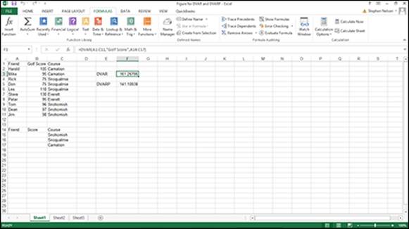
Figure 8-15: Calculate a variance with the DVAR and DVARP functions.
The DVAR function, which appears in cell F3, is
=DVAR(A1:C11,"Golf Score",A14:C17)
and it returns the sample variance of the golf scores shown in the database list for golfers who golf at Snohomish, Snoqualmie, or Carnation. The actual function result is 161.26786.
The DVARP function, which appears in cell F5, is
=DVARP(A1:C11,"Golf Score",A14:C17)
and it returns the population variance of the golf scores shown in the database list for golfers who golf at Snohomish, Snoqualmie, and Carnation. The actual function result is 141.10938.
As when making standard deviation calculations, you don’t simply pick one of the two database variances based on a whim, the weather outside, or how you’re feeling. If you’re calculating a variance using a sample, or subset of items, from the entire data set, or population, you use the DVAR function. To calculate a variance using all the items in the population, you use the DVARP function.
All materials on the site are licensed Creative Commons Attribution-Sharealike 3.0 Unported CC BY-SA 3.0 & GNU Free Documentation License (GFDL)
If you are the copyright holder of any material contained on our site and intend to remove it, please contact our site administrator for approval.
© 2016-2026 All site design rights belong to S.Y.A.