Excel® 2016 Formulas and Functions (2016)
Part II: Harnessing the Power of Functions
10. Working with Date and Time Functions
In This Chapter
How Excel Deals with Dates and Times
Using Excel’s Date Functions
Using Excel’s Time Functions
The date and time functions enable you to convert dates and times to serial numbers and perform operations on those numbers. This capability is useful for such things as accounts receivable aging, project scheduling, time-management applications, and much more. This chapter introduces you to Excel’s date and time functions and puts them through their paces with many practical examples.
How Excel Deals with Dates and Times
Excel uses serial numbers to represent specific dates and times. To get a date serial number, Excel uses December 31, 1899, as an arbitrary starting point and then counts the number of days that have passed since then. For example, the date serial number for January 1, 1900, is 1; for January 2, 1900, it’s 2; and so on. Table 10.1 displays some examples of date serial numbers.
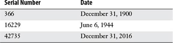
Table 10.1 Examples of Date Serial Numbers
To get a time serial number, Excel expresses time as a decimal fraction of the 24-hour day to get a number between 0 and 1. The starting point, midnight, is given the value 0, so noon—halfway through the day—has a serial number of 0.5. Table 10.2 displays some examples of time serial numbers.
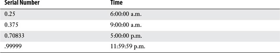
Table 10.2 Examples of Time Serial Numbers
You can combine the two types of serial numbers. For example, 42735.5 represents noon on December 31, 2016.
The advantage of using serial numbers in this way is that it makes calculations involving dates and times very easy. A date or time is really just a number, so any mathematical operation you can perform on a number can also be performed on a date. This is invaluable for worksheets that track delivery times, monitor accounts receivable or accounts payable aging, calculate invoice discount dates, and so on.
Entering Dates and Times
Although it’s true that serial numbers make it easier for the computer to manipulate dates and times, it’s not the best format for humans to comprehend. For example, the number 25404.95555 is meaningless, but the moment it represents (July 20, 1969, at 10:56 p.m. EDT) is one of the great moments in history (the Apollo 11 moon landing). Fortunately, Excel takes care of the conversion between these formats so that you never have to worry about it. To enter a date or time, use any of the formats shown in Table 10.3.
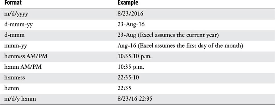
Table 10.3 Excel Date and Time Formats
Tip
Here are a couple shortcuts that will let you enter dates and times quickly. To enter the current date in a cell, press Ctrl+; (semicolon). To enter the current time, press Ctrl+: (colon).
Table 10.3 shows Excel’s built-in formats, but these are not set in stone. You’re free to mix and match these formats, as long as you observe the following rules:
![]() You can use either the forward slash (/) or the hyphen (-) as a date separator. Always use a colon (:) as a time separator.
You can use either the forward slash (/) or the hyphen (-) as a date separator. Always use a colon (:) as a time separator.
![]() You can combine any date and time formats, as long as you separate them with a space.
You can combine any date and time formats, as long as you separate them with a space.
![]() You can enter date and time values using either uppercase or lowercase letters. Excel automatically adjusts the capitalization to its standard format.
You can enter date and time values using either uppercase or lowercase letters. Excel automatically adjusts the capitalization to its standard format.
![]() To display times using the 12-hour clock, include either am (or just a) or pm (or just p). If you leave these off, Excel uses the 24-hour clock.
To display times using the 12-hour clock, include either am (or just a) or pm (or just p). If you leave these off, Excel uses the 24-hour clock.
For more information on formatting dates and times, see “Formatting Numbers, Dates, and Times,” p. 74.
Excel and Two-Digit Years
Entering two-digit years (such as 16 for 2016 and 99 for 1999) is problematic in Excel because various versions of the program treat them differently. In versions since Excel 97, the two-digit years 00 through 29 are interpreted as the years 2000 through 2029, whereas 30 through 99 are interpreted as the years 1930 through 1999. Earlier versions treated the two-digit years 00 through 19 as 2000 through 2019 and 20 through 99 as 1920 through 1999.
Two problems arise here: One is that using a two-digit year such as 25 will cause havoc if the worksheet is loaded into Excel 95 or some earlier version. The second is that you could throw a monkey wrench into your calculations by using a date such as 8/23/30 to mean August 23, 2030 because Excel treats it as August 23, 1930.
The easiest solution to both problems is to always use four-digit years to avoid ambiguity. Alternatively, you can put off the second problem by changing how Excel and Windows interpret two-digit years. Here are the steps to follow in Windows 8, Windows 7, and Windows Vista. (Windows XP and earlier have similar options.)
1. Open Control Panel:
• Windows 8 or later—Press Windows Logo+X and then select Control Panel.
• Windows 7 and Windows Vista—Select Start, Control Panel.
2. Select the Clock, Language, and Region link.
3. Select the Change Date, Time, or Number Formats link. The Region dialog box appears.
4. In the Formats tab, click Additional Settings. (In Vista, click Customize This Format instead.) The Customize Format dialog box appears.
5. Select the Date tab.
6. Use the When a Two-Digit Year Is Entered, Interpret It As a Year Between spinner to adjust the maximum year in which a two-digit year is interpreted as a twenty-first-century date. For example, if you never use dates prior to 1960, you could change the spin box value to 2059, which means Excel interprets two-digit years as dates between 1960 and 2059 (see Figure 10.1).
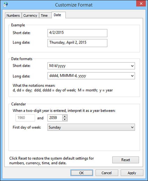
Figure 10.1 Use the Date tab to adjust how Windows (and, therefore, Excel) interprets two-digit years.
7. Click OK to return to the Region dialog box.
8. Click OK to put the new setting into effect.
Using Excel’s Date Functions
Excel’s date functions work with or return date serial numbers. All of Excel’s date-related functions are listed in Table 10.4. (For the serial_number arguments, you can use any valid Excel date.)
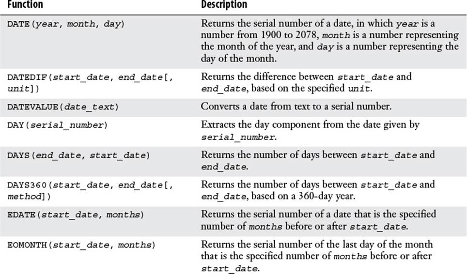
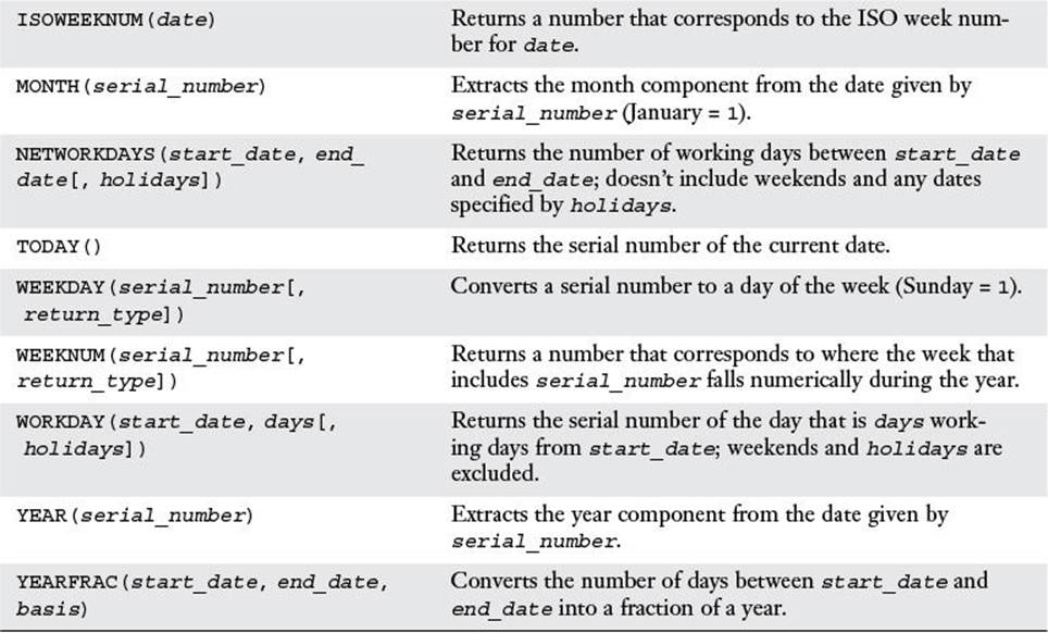
Table 10.4 Excel’s Date Functions
Returning a Date
If you need a date for an expression operand or a function argument, you can enter it by hand if you have a specific date in mind. Much of the time, however, you need more flexibility, such as always entering the current date or building a date from day, month, and year components. Excel offers three functions that can help: TODAY(), DATE(), and DATEVALUE().
TODAY(): Returning the Current Date
When you need to use the current date in a formula, a function, or an expression, use the TODAY() function, which doesn’t take any arguments:
TODAY()
This function returns the serial number of the current date, with midnight as the assumed time. For example, if today’s date is December 31, 2016, the TODAY() function returns the following serial number (although by default, what you see in the cell is the date in m/d/yyyy format):
42735
Note that TODAY() is a dynamic function that doesn’t always return the same value. Each time you edit the formula, enter another formula, recalculate the worksheet, or reopen the workbook, TODAY() updates its value to return the current system date.
DATE(): Returning Any Date
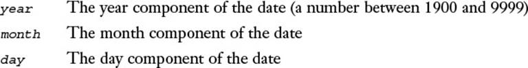
A date consists of three components: the year, month, and day. It often happens that a worksheet generates one or more of these components, and you need some way of building a proper date out of them. You can do that by using Excel’s DATE() function:
DATE(year, month, day)
Caution
Excel’s date inconsistencies rear up again with the DATE() function. That’s because, if you enter a two-digit year (or even a three-digit year), Excel converts the number into a year value by adding 1900. So, entering 16 as the year argument gives you 1916, not 2016. To avoid problems, always use a four-digit year when entering the DATE() function’s year argument.
For example, the following expression returns Christmas Day in 2016:
DATE(2016, 12, 25)
Note, too, that DATE() adjusts for wrong month and day values. For example, the following expression returns January 1, 2017:
DATE(2016, 12, 32)
Here, DATE() adds the extra day (there are 31 days in December) to return the date of the next day. Similarly, the following expression returns January 25, 2017:
DATE(2016, 13, 25)
DATEVALUE(): Converting a String to a Date
If you have a date value in string form, you can convert it to a date serial number by using the DATEVALUE() function:
DATEVALUE(date_text)
![]()
For example, the following expression returns the date serial number for the string August 23, 2016:
DATEVALUE("August 23, 2016")
![]() To learn how to convert nonstandard date strings to dates, see “A Date-Conversion Formula,” p. 154.
To learn how to convert nonstandard date strings to dates, see “A Date-Conversion Formula,” p. 154.
Returning Parts of a Date
The three components of a date—year, month, and day—can also be extracted individually from a given date. This might not seem all that interesting at first, but actually many useful techniques arise out of working with a date’s component parts. A date’s components are extracted using Excel’s YEAR(), MONTH(), and DAY() functions.
The YEAR() Function
The YEAR() function returns a four-digit number that corresponds to the year component of a specified date:
YEAR(serial_number)
![]()
For example, if today is August 23, 2016, the following expression will return 2016:
YEAR(TODAY())
The MONTH() Function
The MONTH() function returns a number between 1 and 12 that corresponds to the month component of a specified date:
MONTH(serial_number)
![]()
For example, the following expression returns 8:
MONTH("August 23, 2016")
The DAY() Function
The DAY() function returns a number between 1 and 31 that corresponds to the day component of a specified date:
DAY(serial_number)
![]()
For example, the following expression returns 23:
DAY("8/23/2016")
The WEEKDAY() Function
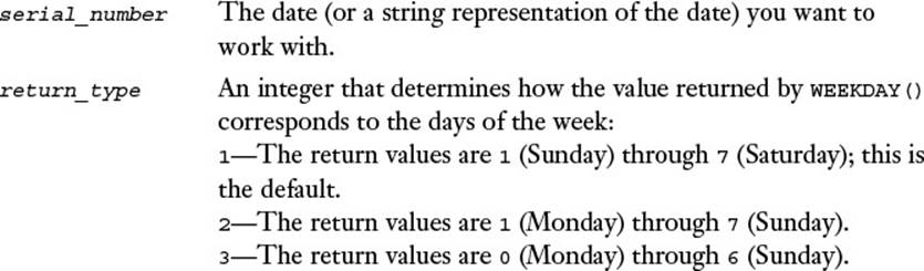
The WEEKDAY() function returns a number that corresponds to the day of the week upon which a specified date falls:
WEEKDAY(serial_number[, return_type])
For example, the following expression returns 3 because August 23, 2016, is a Tuesday:
WEEKDAY("8/23/2016")
![]() To learn how to use CHOOSE() to convert the WEEKDAY() return value into a day name, see “Determining the Name of the Day of the Week,” p. 194.
To learn how to use CHOOSE() to convert the WEEKDAY() return value into a day name, see “Determining the Name of the Day of the Week,” p. 194.
The WEEKNUM() Function
The WEEKNUM() function returns a number that corresponds to where the week that includes a specified date falls numerically during the year:
WEEKNUM(serial_number[, return_type])
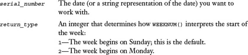
For example, the following expression returns 35 because August 23, 2016, falls in the 35th week of 2016:
WEEKNUM("August 23, 2016")
Tip
You might need to return a week number that corresponds to ISO (International Standards Organization) 8601, which is the international standard for the representation of dates and times. The ISO 8601 week-numbering year always begins on the week with the year’s first Thursday, so there will be dates at the beginning of the year and the end of the year where the ISO week number differs from the calendar week number. To always return the ISO week number, use Excel’s ISOWEEKNUM(date) function (where date is the date you want to work with).
Returning a Date X Years, Months, or Days from Now
You can take advantage of the fact that, as I mentioned earlier, DATE() automatically adjusts wrong month and day values by applying formulas to one or more of the DATE() function’s arguments. The most common use for this is returning a date that occurs X number of years, months, or days from now (or from any date).
For example, suppose that you want to know which day of the week the 4th of July falls on next year. Here’s a formula that figures it out:
=WEEKDAY(DATE(YEAR(TODAY())) + 1, 7, 4)
As another example, if you want to work with whatever date is 6 months from today, you would use the following expression:
DATE(YEAR(TODAY()), MONTH(TODAY()) + 6, DAY(TODAY()))
Given this technique, you’ve probably figured out that you can return a date that is X days from now (or whenever) by adding to the day component of the DATE() function. For example, here’s an expression that returns a date 30 days from now:
DATE(YEAR(TODAY()), MONTH(TODAY()), DAY(TODAY() + 30))
This is overkill, however, because date addition and subtraction works at the day level in Excel. That is, if you simply add or subtract a number to or from a date, Excel adds or subtracts that number of days. For example, to return a date 30 days from now, you need only use the following expression:
TODAY() + 30
A Workday Alternative: The WORKDAY() Function
Adding days to or subtracting days from a date is straightforward, but the basic calculation includes all days: workdays, weekends, and holidays. In many cases, you might need to ignore weekends and holidays and return a date that is a specified number of workdays from some original date.
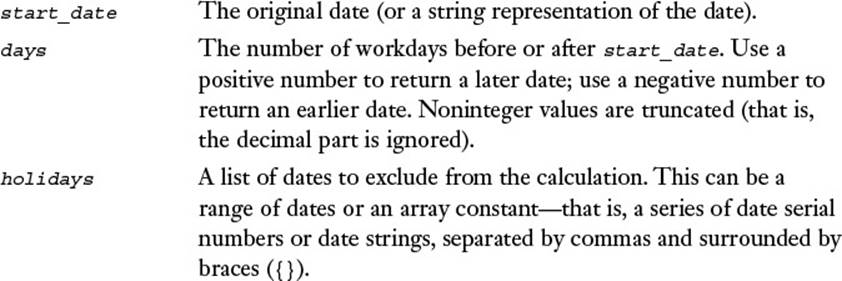
You can do this by using the WORKDAY() function, which returns a date that is a specified number of working days from some starting date:
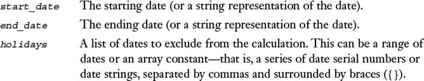
WORKDAY(start_date, days[, holidays])
For example, the following expression returns a date that is 30 workdays from today:
WORKDAY(TODAY(), 30)
Here’s another expression that returns the date that is 30 workdays from December 1, 2016, excluding December 25, 2016, and January 1, 2017:
=WORKDAY("12/1/2016", 30, {"12/25/2016","1/1/2017"})
![]() It’s possible to calculate the various holidays that occur within a year and place the dates within a range for use as the WORKDAY() function’s holidays argument. See “Calculating Holiday Dates”, p. 221.
It’s possible to calculate the various holidays that occur within a year and place the dates within a range for use as the WORKDAY() function’s holidays argument. See “Calculating Holiday Dates”, p. 221.
Adding X Months: A Problem
You should be aware that simply adding X months to a specified date’s month component won’t always return the result you expect. The problem is that the months have a varying number of days. So, if you add a certain number of months to a date that falls on or near the end of a month, and the future month does not have the same number of days, Excel adjusts the day component accordingly.
For example, suppose that A1 contains the date 1/31/2017, and consider the following formula:
=DATE(YEAR(A1), MONTH(A1) + 3, DAY(A1))
You might expect this formula to return the last date in April as the result. Unfortunately, adding three months returns the wrong date, 4/31/2017 (there are only 30 days in April), which Excel automatically converts to 5/1/2017.
You can avoid this problem by using two functions: EDATE() and EOMONTH().
The EDATE() Function
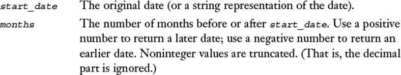
The EDATE() function returns a date that is the specified number of months before or after a starting date:
EDATE(start_date, months)
The nice thing about the EDATE() function is that it performs a “smart” calculation when working with dates at or near the end of the month: If the day component of the returned date doesn’t exist (for example, April 31), EDATE() returns the last day of the month (April 30).
The EDATE() function is useful for calculating the coupon payment dates for bond issues. Given the bond’s maturity date, you calculate the bond’s first payment as follows (assuming that the bond was issued this year and that the maturity date is in a cell named MaturityDate):
=DATE(YEAR(TODAY()), MONTH(MaturityDate), DAY(MaturityDate))
If this result is in cell A1, the following formula will return the date of the next coupon payment:
=EDATE(A1, 6)
The EOMONTH() Function
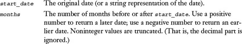
The EOMONTH() function returns the date of the last day of the month that is the specified number of months before or after a starting date:
EOMONTH(start_date, months)
For example, the following formula returns the last day of the month three months from now:
=EOMONTH(TODAY(), 3)
Returning the Last Day of Any Month
The EOMONTH() function returns the last date of some month in the future or the past. However, what if you have a date, and you want to know the last day of the month in which that date appears?
You can calculate this by using yet another trick involving the DATE() function’s capability to adjust wrong values for date components. You want a formula that returns the last day of a particular month. You can’t specify the day argument in the DATE() function directly because the months can have 28, 29, 30, or 31 days. Instead, you can take advantage of an apparently trivial fact: The last day of any month is always the day before the first day of the next month. The number before 1 is 0, so you can plug in 0 to the DATE() function as the day argument:
=DATE(YEAR(MyDate), MONTH(MyDate) + 1, 0)
Here, assume that MyDate is the date you want to work with.
Determining a Person’s Birthday, Given the Birth Date
If you know a person’s birth date, determining that person’s birthday is easy: Just keep the month and day the same and substitute the current year for the year of birth. To accomplish this in a formula, you could use the following:
=DATE(YEAR(NOW()), MONTH(Birthdate), DAY(Birthdate))
Here, I’m assuming that the person’s date of birth is in a cell named Birthdate. The YEAR(NOW()) component extracts the current year, and MONTH(Birthdate) and DAY(Birthdate) extract the month and day, respectively, from the person’s date of birth. Combine these into theDATE() function, and you have the birthday.
Returning the Date of the nth Occurrence of a Weekday in a Month
It’s a common date task to have to figure out the nth weekday in a given month. For example, you might need to schedule a budget meeting for the first Monday in each month, or you might want to plan the annual company picnic for the third Sunday in June. These are tricky calculations, to be sure, but Excel’s date functions are up to the task.
As with many other complex formulas, the best place to start is with what you know for sure. In this case, you always know for sure the date of the first day of whatever month you’re dealing with. For example, Labor Day always occurs on the first Monday in September, so you could begin with September 1 and know that the date you seek is some number of days after that. The formula begins like this:
=DATE(Year, Month, 1) + days
Here, Year is the year in which you want the date to fall, and Month is the number of the month you want to work with. The days value is what you need to calculate.
To simplify things for now, let’s assume that you’re trying to find a date that is the first occurrence of a particular weekday in a month (such as Labor Day, the first Monday in September).
Using the first of the month as your starting point, you need to ask whether the weekday you’re working with is less than the weekday of the first of the month. (By “less than,” I mean that the WEEKDAY() value of the day of the week you’re working with is numerically smaller than theWEEKDAY() value the first of the month.) In the Labor Day example, September 1, 2016, falls on a Thursday (WEEKDAY() equals 5), which is greater than Monday (WEEKDAY() equals 2). The result of this comparison determines how many days you add to the 1st to get the date you seek:
![]() If the day of the week you’re working with is less than the first of the month, the date you seek is the first plus the result of the following expression:
If the day of the week you’re working with is less than the first of the month, the date you seek is the first plus the result of the following expression:
7 - WEEKDAY(DATE(Year, Month, 1)) + Weekday
Here, Weekday is the WEEKDAY() value of the day of the week you’re working with. Here’s the expression for the Labor Day example:
7 - WEEKDAY(DATE(2016, 9, 1)) + 2
![]() If the day of the week you’re working with is greater than or equal to the first of the month, the date you seek is the first plus the result of the following expression:
If the day of the week you’re working with is greater than or equal to the first of the month, the date you seek is the first plus the result of the following expression:
Weekday - WEEKDAY(DATE(Year, Month, 1))
Again, Weekday is the WEEKDAY() value of the day of the week you’re working with. Here’s the expression for the Labor Day example:
2 - WEEKDAY(DATE(2016, 9, 1))
These conditions can be handled by a basic IF() function. Here, then, is the generic formula for calculating the first occurrence of a Weekday in a given Year and Month:
=DATE(Year, Month, 1) + IF(Weekday < WEEKDAY(DATE(Year, Month, 1)), 7 - WEEKDAY(DATE(Year, Month, 1)) + Weekday, Weekday - WEEKDAY(DATE(Year, Month, 1)))
Here’s the formula for calculating the date of Labor Day in 2016:
=DATE(2016, 9, 1) + IF(2 < WEEKDAY(DATE(2016, 9, 1)), 7 - WEEKDAY(DATE(2016, 9, 1)) + 2, 2 - WEEKDAY(DATE(2016, 9, 1)))
Generalizing this formula for the nth occurrence of a weekday is straightforward: The second occurrence comes one week after the first, the third occurrence comes two weeks after the first, and so on. Here’s a generic expression to calculate the extra number of days to add (where n is an integer that represents the nth occurrence):
(n - 1) * 7
Here, then, in generic form, is the final formula for calculating the nth occurrence of a Weekday in a given Year and Month:
=DATE(Year, Month, 1) + IF(Weekday < WEEKDAY(DATE(Year, Month, 1)), 7 - WEEKDAY(DATE(Year, Month, 1)) + Weekday, Weekday - WEEKDAY(DATE(Year, Month, 1))) + (n - 1) * 7
For example, the following formula calculates the date of the third Sunday (WEEKDAY() equals 1) in June for 2016:
=DATE(2016, 6, 1) + IF(1 < WEEKDAY(DATE(2016, 6, 1)), 7 - WEEKDAY(DATE(2016, 6, 1)) + 1,
[ic:ccc]1 - WEEKDAY(DATE(2016, 6, 1))) +
[ic:ccc](3 - 1) * 7
Figure 10.2 shows a worksheet used for calculating the nth occurrence of a weekday.
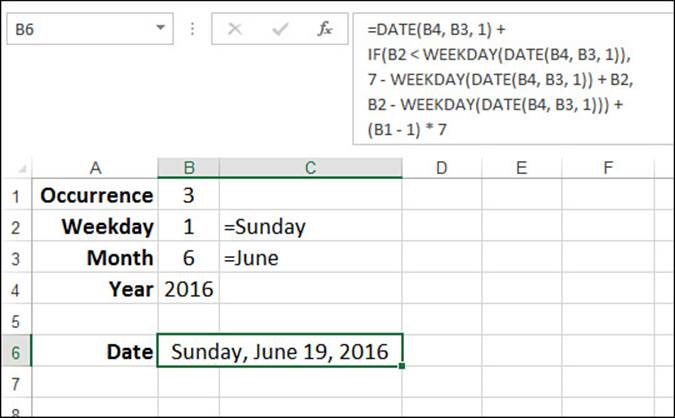
Figure 10.2 This worksheet calculates the nth occurrence of a specified weekday in a given year and month.
Note
You can download this chapter’s sample workbook at www.mcfedries.com/books/book.php?title=excel-2016-formulas-and-functions.
The input cells are as follows:
![]() B1—The number of the occurrence.
B1—The number of the occurrence.
![]() B2—The number of the weekday. (The formula in C2 shows the name of the entered weekday.)
B2—The number of the weekday. (The formula in C2 shows the name of the entered weekday.)
![]() B3—The number of the month. (The formula in C3 shows the name of the entered month.)
B3—The number of the month. (The formula in C3 shows the name of the entered month.)
![]() B4—The year.
B4—The year.
The date calculation appears in cell B6. Here’s the formula:
=DATE(B4, B3, 1) + IF(B2 < WEEKDAY(DATE(B4, B3, 1)), 7 - WEEKDAY(DATE(B4, B3, 1)) + B2, B2 - WEEKDAY(DATE(B4, B3, 1))) + (B1 - 1) * 7
Calculating Holiday Dates
Given the formula from the previous section, it becomes a relative breeze to calculate the dates for most floating holidays (that is, holidays that occur on the nth weekday of a month instead of on a specific date each year, as do holidays such as Christmas, Independence Day, and Canada Day).
Here are the standard statutory floating holidays in the United States:
![]() Martin Luther King Jr. Day—Third Monday in January
Martin Luther King Jr. Day—Third Monday in January
![]() Presidents Day—Third Monday in February
Presidents Day—Third Monday in February
![]() Memorial Day—Last Monday in May
Memorial Day—Last Monday in May
![]() Labor Day—First Monday in September
Labor Day—First Monday in September
![]() Columbus Day—Second Monday in October
Columbus Day—Second Monday in October
![]() Thanksgiving Day—Fourth Thursday in November
Thanksgiving Day—Fourth Thursday in November
Here’s the list for Canada:
![]() Victoria Day—Monday on or before May 24
Victoria Day—Monday on or before May 24
![]() Good Friday—Friday before Easter Sunday
Good Friday—Friday before Easter Sunday
![]() Labor Day—First Monday in September
Labor Day—First Monday in September
![]() Thanksgiving Day—Second Monday in October
Thanksgiving Day—Second Monday in October
Figure 10.3 shows a worksheet used to calculate the holiday dates in a specified year.
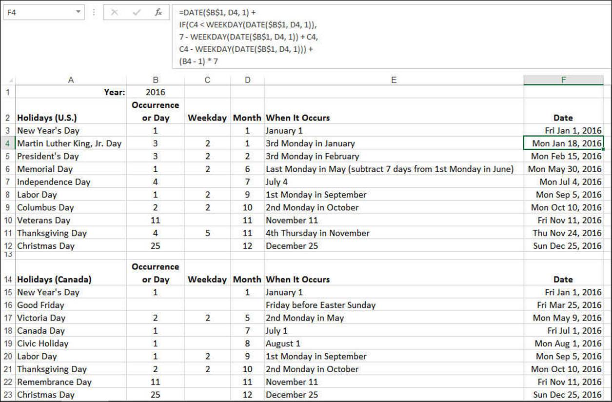
Figure 10.3 This worksheet calculates the dates of numerous holidays in a given year.
Column A holds the name of the holiday; column B holds the occurrence within the month or, for fixed holidays, the actual date within the month; column C holds the days of the week; and column D holds the number of the month.
Most of the values in column E are calculated. For the floating holidays, for example, several CHOOSE() functions are used to construct the description. Here’s an example for Martin Luther King, Jr., Day:
=B5 & CHOOSE(B5, "st", "nd", "rd", "th", "th") & " " & CHOOSE(C5, "Sunday", "Monday", "Tuesday", "Wednesday", "Thursday", "Friday", "Saturday") & " in " & CHOOSE(D5, "January", "February", "March", "April", "May", "June", "July", "August", "September", "October", "November", "December")
Finally, column F contains the formulas for calculating the date of each holiday based on the year entered in cell B1.
Note
Two exceptions exist in column F. The first is the formula for Memorial Day (cell F6), which occurs on the last Monday in May. To derive this date, you first calculate the first Monday in June and then subtract 7 days.
The second exception is the formula for Good Friday (cell F16). This occurs two days before Easter Sunday, which is a floating holiday, but its date is based on the phase of the moon, of all things. (Officially, Easter Sunday falls on the first Sunday after the first ecclesiastical full moon after the spring equinox.) There are no simple formulas for calculating when Easter Sunday occurs in a given year. The formula in the Holidays worksheet is a complex bit of business that uses the FLOOR() function, so I discuss it when I discuss that function inChapter 11, “Working with Math Functions.”
Calculating the Julian Date
Excel has built-in functions that convert a given date into a numerical day of the week (the WEEKDAY() function) and that return the numerical ranking of the week in which a given date falls (the WEEKNUM() function). However, Excel doesn’t have a function that calculates the Julian date for a given date—the numerical ranking of the date for the year in which it falls. For example, the Julian date of January 1 is 1, January 2 is 2, and February 1 is 32.
If you need to use Julian dates in your business, here’s a formula that will do the job:
=MyDate - DATE(YEAR(MyDate) - 1, 12, 31)
This formula assumes that the date you want to work with is in a cell named MyDate. The expression DATE(YEAR(MyDate) - 1, 12, 31) returns the date serial number for December 31 of the preceding year. Subtracting this number from MyDate gives you the Julian number.
Calculating the Difference Between Two Dates
In the previous section, you saw that Excel enables you to subtract one date from another. Here’s an example:
=Date1 - Date2
Here, Date1 and Date2 can be date values or date strings. When you create such a formula, Excel returns a value equal to the number of days between the two dates. This date-difference formula returns a positive number if Date1 is larger than Date2; it returns a negative number ifDate1 is less than Date2. Calculating the difference between two dates is useful in many business scenarios, including receivables aging, interest calculations, benefits payments, and more.
Note
If you enter a simple date-difference formula in a cell, Excel automatically formats that cell as a date. For example, if the difference between the two days is 30 days, you see 1/30/1900 as the result. (If the result is negative, you see the cell filled with # symbols.) To see the result properly, you need to format the cell with the General format or some numeric format.
Besides the basic date-difference formula, you can use the date functions from earlier in this chapter to perform date-difference calculations. Also, Excel boasts a number of worksheet functions that enable you to perform more sophisticated operations to determine the difference between two dates. The rest of this section runs through a number of these date-difference formulas and functions.
Calculating a Person’s Age, Part I
If you have a person’s birth date entered into a cell named Birthdate and you need to calculate how old the person is, you might think that the following formula would do the job:
=YEAR(TODAY()) - YEAR(Birthdate)
This works, but only if the person’s birthday has already passed this year. If he hasn’t had a birthday yet, this formula reports the age as being one year greater than it really is.
To solve this problem, you need to take into account whether the person’s birthday has passed. To see how to do this, check out the following logical expression:
=DATE(YEAR(NOW()), MONTH(Birthdate), DAY(Birthdate)) > TODAY()
This expression asks whether the person’s birthday for this year (which uses the formula from earlier in this chapter—see “Determining a Person’s Birthday, Given the Birth Date”) is greater than today’s date. If it is, the expression returns logical TRUE, which is equivalent to 1; if it isn’t, the expression returns logical FALSE, which is equivalent to 0. In other words, you can get the person’s true age by subtracting the result of the logical expression from the original formula, like so:
=YEAR(NOW()) - YEAR(Birthdate) - (DATE(YEAR(NOW()), MONTH(Birthdate), DAY(Birthdate)) > NOW())
DAYS(): Returning the Number of Days Between Two Dates
If all you’re interested in is the number of days between two dates, then the easiest way to perform such a calculation is to use Excel’s DAYS() function:
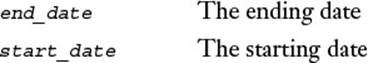
DAYS(end_date, start_date)
For example, the following formula returns the number of days that have elapsed since the start of the current year:
=DAYS(TODAY(), DATE(YEAR(TODAY(), 1, 1))
The DATEDIF() Function
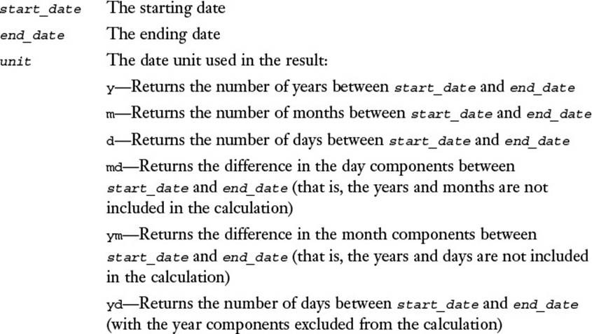
If you need to perform date-difference calculations based on a date unit other than days, then you need to use the DATEDIF() function, which returns the difference between two specified dates, based on a specified unit:
DATEDIF(start_date, end_date[, unit])
You can use the DATEDIF() function to perform a Julian date calculation, as explained earlier in this chapter (see “Calculating the Julian Date”). If the date you want to work with is in a cell named MyDate, the following formula calculates its Julian date using DATEDIF():
=DATEDIF(DATE(YEAR(MyDate) - 1, 12, 31), MyDate, "d")
Caution
DATEDIF() is an undocumented Excel function because it was plagued with errors in earlier versions of Excel. Use this function with caution, and avoid using it altogether on very important worksheets.
Calculating a Person’s Age, Part II
The DATEDIF() function can greatly simplify the formula for calculating a person’s age. (See “Calculating a Person’s Age, Part I,” earlier in this chapter.) If the person’s date of birth is in a cell named Birthdate, the following formula calculates his current age:
=DATEDIF(Birthdate, TODAY(), "y")
NETWORKDAYS(): Calculating the Number of Workdays Between Two Dates
If you calculate the difference in days between two days, Excel includes weekends and holidays. In many business situations, you need to know the number of workdays between two dates. For example, when calculating the number of days an invoice is past due, it’s often best to exclude weekends and holidays.
This is easily done using the NETWORKDAYS() function (read the name as net workdays), which returns the number of working days between two dates:
NETWORKDAYS(start_date, end_date[, holidays])
For example, here’s an expression that returns the number of workdays between December 1, 2016, and January 10, 2017, excluding December 25, 2016, and January 1, 2017:
=NETWORKDAYS("12/1/2016", "1/10/2017", {"12/25/2016","1/1/2017"})
Figure 10.4 shows an update to the accounts receivable worksheet that uses NETWORKDAYS() to calculate the number of workdays that each invoice is past due.
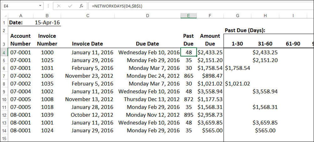
Figure 10.4 This worksheet calculates the number of workdays that each invoice is past due by using the NETWORKDAYS() function.
DAYS360(): Calculating Date Differences Using a 360-Day Year
Many accounting systems operate using the principle of a 360-day year, which divides the year into 12 periods of uniform (30-day) lengths. Finding the number of days between dates in such a system isn’t possible with the standard addition and subtraction of dates. However, Excel makes such calculations easy with its DAYS360() function, which returns the number of days between a starting date and an ending date, based on a 360-day year:
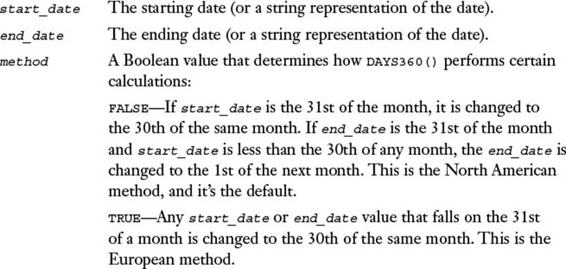
DAYS360(start_date, end_date[, method])
For example, the following expression returns the value 1:
DAYS360("3/30/2016", "4/1/2016")
YEARFRAC(): Returning the Fraction of a Year Between Two Dates
Business worksheet models often need to know the fraction of a year that has elapsed between one date and another. For example, if an employee leaves after 3 months, you might need to pay out a quarter of a year’s worth of benefits. This calculation can be complicated by the fact that your company might use a 360-day accounting year. However, the YEARFRAC() function can help you. This function converts the number of days between a start date and an end date into a fraction of a year:
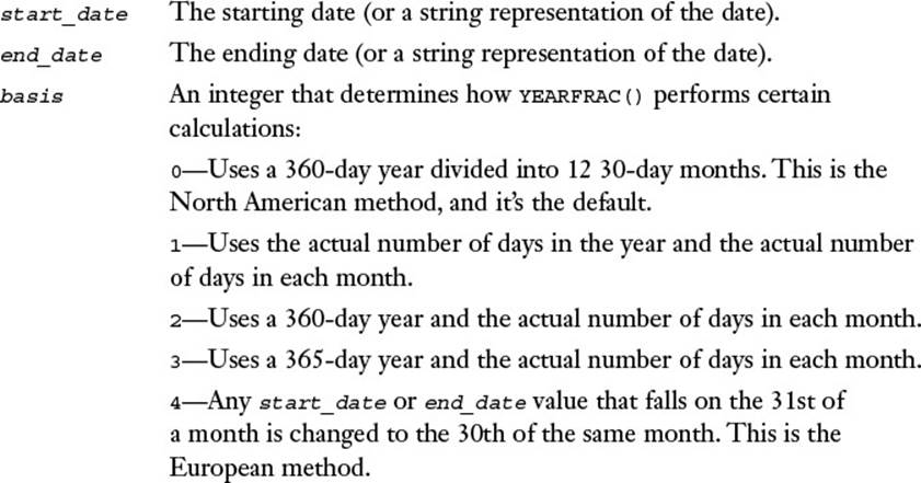
YEARFRAC(start_date, end_date[, basis])
For example, the following expression returns the value 0.25:
YEARFRAC("3/15/2016", "6/15/2016")
Using Excel’s Time Functions
Working with time values in Excel is not greatly different from working with date values, although there are some exceptions, as you’ll see in this section. Here you’ll work mostly with Excel’s time functions, which work with or return time serial numbers. All of Excel’s time-related functions are listed in Table 10.5. (For the serial_number arguments, you can use any valid Excel time.)
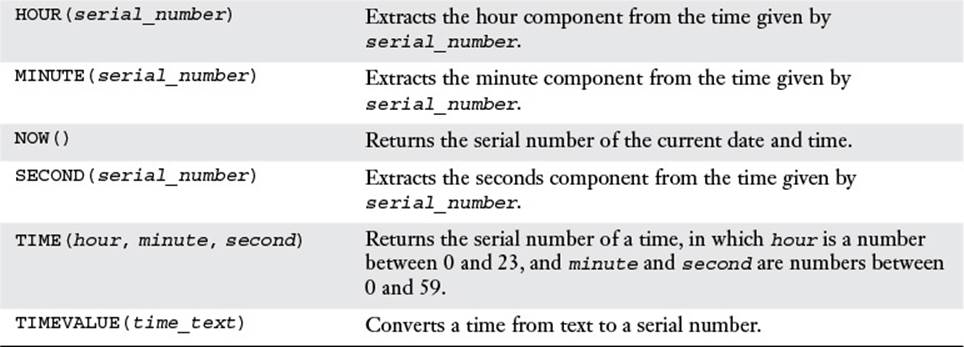
Table 10.5 Excel’s Time FunctionsFunction Description
Returning a Time
If you need a time value to use in an expression or a function, either you can enter it by hand if you have a specific date that you want to work with, or you can take advantage of the flexibility of three Excel functions: NOW(), TIME(), and TIMEVALUE().
NOW(): Returning the Current Time
When you need to use the current time in a formula, a function, or an expression, use the NOW() function, which doesn’t take any arguments:
NOW()
This function returns the serial number of the current time, with the current date as the assumed date. For example, if it’s noon and today’s date is December 31, 2016, the NOW() function returns the following serial number (although in the cell you see this displayed using the m/d/yyyy h:mm format):
42735.5
If you just want the time component of the serial number, subtract TODAY() from NOW():
NOW() - TODAY()
Just like the TODAY() function, remember that NOW() is a dynamic function that doesn’t keep its initial value (that is, the time at which you entered the function). Each time you edit the formula, enter another formula, recalculate the worksheet, or reopen the workbook, NOW() uptimes its value to return the current system time.
TIME(): Returning Any Time
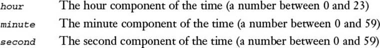
A time consists of three components: the hour, minute, and second. It often happens that a worksheet generates one or more of these components, and you need some way of building a proper time out of them. You can do that by using Excel’s TIME() function:
TIME(hour, minute, second)
For example, the following expression returns the time 2:45:30 p.m.:
TIME(14, 45, 30)
Like the DATE() function, TIME() adjusts for wrong hour, month, and second values. For example, the following expression returns 3:00:30 p.m.:
TIME(14, 60, 30)
Here, TIME() takes the extra minute and adds 1 to the hour value.
TIMEVALUE(): Converting a String to a Time
If you have a time value in string form, you can convert it to a time serial number by using the TIMEVALUE() function:
TIMEVALUE(time_text)
![]()
For example, the following expression returns the time serial number for the string 2:45:00 PM:
TIMEVALUE("2:45:00 PM")
Returning Parts of a Time
The three components of a time—hour, minute, and second—can also be extracted individually from a given time, using Excel’s HOUR(), MINUTE(), and SECOND() functions.
The HOUR() Function
The HOUR() function returns a number between 0 and 23 that corresponds to the hour component of a specified time:
HOUR(serial_number)
![]()
For example, the following expression returns 12:
HOUR(0.5)
The MINUTE() Function
The MINUTE() function returns a number between 0 and 59 that corresponds to the minute component of a specified time:
MINUTE(serial_number)

For example, if it’s currently 3:15 p.m., the following expression returns 15:
MINUTE(NOW())
The SECOND() Function
The SECOND() function returns a number between 0 and 59 that corresponds to the second component of a specified time:
SECOND(serial_number)
![]()
For example, the following expression returns 30:
SECOND("2:45:30 PM")
Returning a Time X Hours, Minutes, or Seconds from Now
As I mentioned earlier, TIME() automatically adjusts wrong hour, minute, and second values. You can take advantage of this by applying formulas to one or more of the TIME() function’s arguments. The most common use for this is to return a time that occurs X number of hours, minutes, or seconds from now (or from any time).
For example, the following expression returns the time 12 hours from now:
TIME(HOUR(NOW()) + 12, MINUTE(NOW()), SECOND(NOW()))
Unlike the DATE() function, the TIME() function doesn’t enable you to simply add an hour, a minute, or a second to a specified time. For example, consider the following expression:
NOW() + 1
All this does is add 1 day to the current date and time.
If you want to add hours, minutes, and seconds to a time, you need to express the added time as a fraction of a day. For example, because there are 24 hours in a day, 1 hour is represented by the expression 1/24. Similarly, because there are 60 minutes in an hour, 1 minute is represented by the expression 1/24/60. Finally, because there are 60 seconds in a minute, 1 second is represented by the expression 1/24/60/60. Table 10.6 shows you how to use these expressions to add n hours, minutes, and seconds.
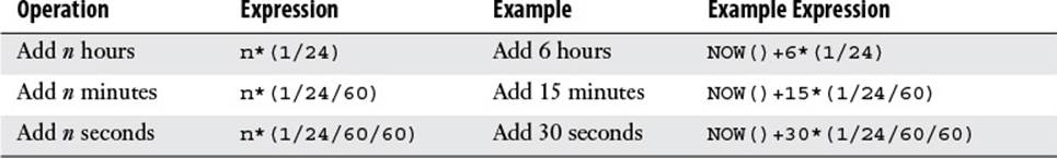
Table 10.6 Adding Hours, Minutes, and Seconds
Summing Time Values
When working with time values in Excel, you need to be aware that there are two subtly different interpretations for the phrase “adding one time to another”:
![]() Adding time values to get a future time—As you saw in the previous section, adding hours, minutes, or seconds to a time returns a value that represents a future time. For example, if the current time is 11:00 p.m. (23:00), adding 2 hours returns the time 1:00 a.m.
Adding time values to get a future time—As you saw in the previous section, adding hours, minutes, or seconds to a time returns a value that represents a future time. For example, if the current time is 11:00 p.m. (23:00), adding 2 hours returns the time 1:00 a.m.
![]() Adding time values to get a total time—In this interpretation, time values are summed to get a total number of hours, minutes, and seconds. This is useful if you want to know how many hours an employee worked in a week or how many hours to bill a client. In this case, for example, if the current total is 23 hours, adding 2 hours brings the total to 25 hours.
Adding time values to get a total time—In this interpretation, time values are summed to get a total number of hours, minutes, and seconds. This is useful if you want to know how many hours an employee worked in a week or how many hours to bill a client. In this case, for example, if the current total is 23 hours, adding 2 hours brings the total to 25 hours.
The problem is that adding time values to get a future time is Excel’s default interpretation for added time values. So, if cell A1 contains 23:00 and cell A2 contains 2:00, the following formula returns 1:00:00 AM:
=A1 + A2
The time value 25:00:00 is stored internally, but Excel adjusts the display so that you see the “correct” value 1:00:00 AM. If you want to see 25:00:00 instead, apply the following custom format to the cell:
[h]:mm:ss
Calculating the Difference Between Two Times
Excel treats time serial numbers as decimal expansions (numbers between 0 and 1) that represent fractions of a day. Because they’re just numbers, there’s nothing to stop you from subtracting one from another to determine the difference between them:
EndTime - StartTime
This expression works just fine, as long as EndTime is greater than StartTime. (I used the names EndTime and StartTime purposefully so you’d remember to always subtract the later time from the earlier time.)
However, there’s one scenario in which this expression fails: If EndTime occurs after midnight the next day, there’s a good chance that it will be less than StartTime. For example, if a person works from 11:00 p.m. to 7:00 a.m., the expression 7:00 AM - 11:00 PM results in an illegal negative time value. (Excel displays the result as a series of # symbols that fill the cell.)
To ensure that you get the correct positive result in this situation, use the following generic expression:
IF(EndTime < StartTime, 1 + EndTime - StartTime, EndTime - StartTime)
The IF() function checks to see whether EndTime is less than StartTime. If it is, 1 is added to the value EndTime - StartTime to get the correct result; otherwise, just EndTime - StartTime is returned.
Case Study: Building an Employee Time Sheet
In this case study, you’ll put your new knowledge of time functions and calculations to good use building a time sheet that tracks the number of hours an employee works each week, takes into account hours worked on weekends and holidays, and calculates the total number of hours and the weekly pay. Figure 10.5 shows the completed time sheet.
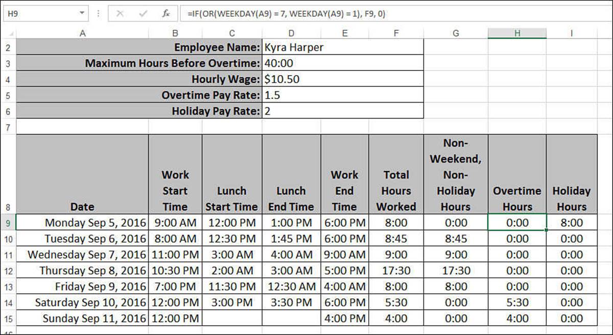
Figure 10.5 This employee time sheet tracks the daily hours, takes weekends and holidays into account, and calculates the employee’s total working hours and pay.
Before starting, you need to understand three terms used in this case study:
![]() Regular hours—These are hours worked for regular pay.
Regular hours—These are hours worked for regular pay.
![]() Overtime hours—These are hours worked beyond the maximum number of regular hours, as well as any hours worked on the weekend.
Overtime hours—These are hours worked beyond the maximum number of regular hours, as well as any hours worked on the weekend.
![]() Holiday hours—These are hours worked on a statutory holiday.
Holiday hours—These are hours worked on a statutory holiday.
Entering the Time Sheet Data
Let’s begin at the top of the time sheet, where the following data is required:
![]() Employee Name—You’ll create a separate sheet for each employee, so enter the person’s name here. You might also want to augment this with the date the person started or other data about the employee.
Employee Name—You’ll create a separate sheet for each employee, so enter the person’s name here. You might also want to augment this with the date the person started or other data about the employee.
![]() Maximum Hours Before Overtime—This is the number of regular hours an employee has to work in a week before overtime hours take effect. Enter the number using the hh:mm format. Cell D3 uses the [h]:mm custom format, to ensure that Excel displays the actual value.
Maximum Hours Before Overtime—This is the number of regular hours an employee has to work in a week before overtime hours take effect. Enter the number using the hh:mm format. Cell D3 uses the [h]:mm custom format, to ensure that Excel displays the actual value.
![]() Hourly Wage—This is the amount the employee earns per regular hour of work.
Hourly Wage—This is the amount the employee earns per regular hour of work.
![]() Overtime Pay Rate—This is the factor by which the employee’s hourly rate is increased for overtime hours. For example, enter 1.5 if the employee earns time and a half for overtime.
Overtime Pay Rate—This is the factor by which the employee’s hourly rate is increased for overtime hours. For example, enter 1.5 if the employee earns time and a half for overtime.
![]() Holiday Pay Rate—This is the factor by which the employee’s hourly rate is increased for holiday hours. For example, enter 2 if the employee earns double time for holidays.
Holiday Pay Rate—This is the factor by which the employee’s hourly rate is increased for holiday hours. For example, enter 2 if the employee earns double time for holidays.
Calculating the Daily Hours Worked
Figure 10.6 shows the portion of the time sheet used to record the employee’s daily hours worked. For each day, you enter five items:
![]() Date—Enter the date the employee worked. This is formatted to show the day of the week, which is useful for confirming overtime hours worked on weekends.
Date—Enter the date the employee worked. This is formatted to show the day of the week, which is useful for confirming overtime hours worked on weekends.
![]() Work Start Time—Enter the time of day the employee began working.
Work Start Time—Enter the time of day the employee began working.
![]() Lunch Start Time—Enter the time of day the employee stopped for lunch.
Lunch Start Time—Enter the time of day the employee stopped for lunch.
![]() Lunch End Time—Enter the time of day the employee resumed working after lunch.
Lunch End Time—Enter the time of day the employee resumed working after lunch.
![]() Work End Time—Enter the time of day the employee stopped working.
Work End Time—Enter the time of day the employee stopped working.
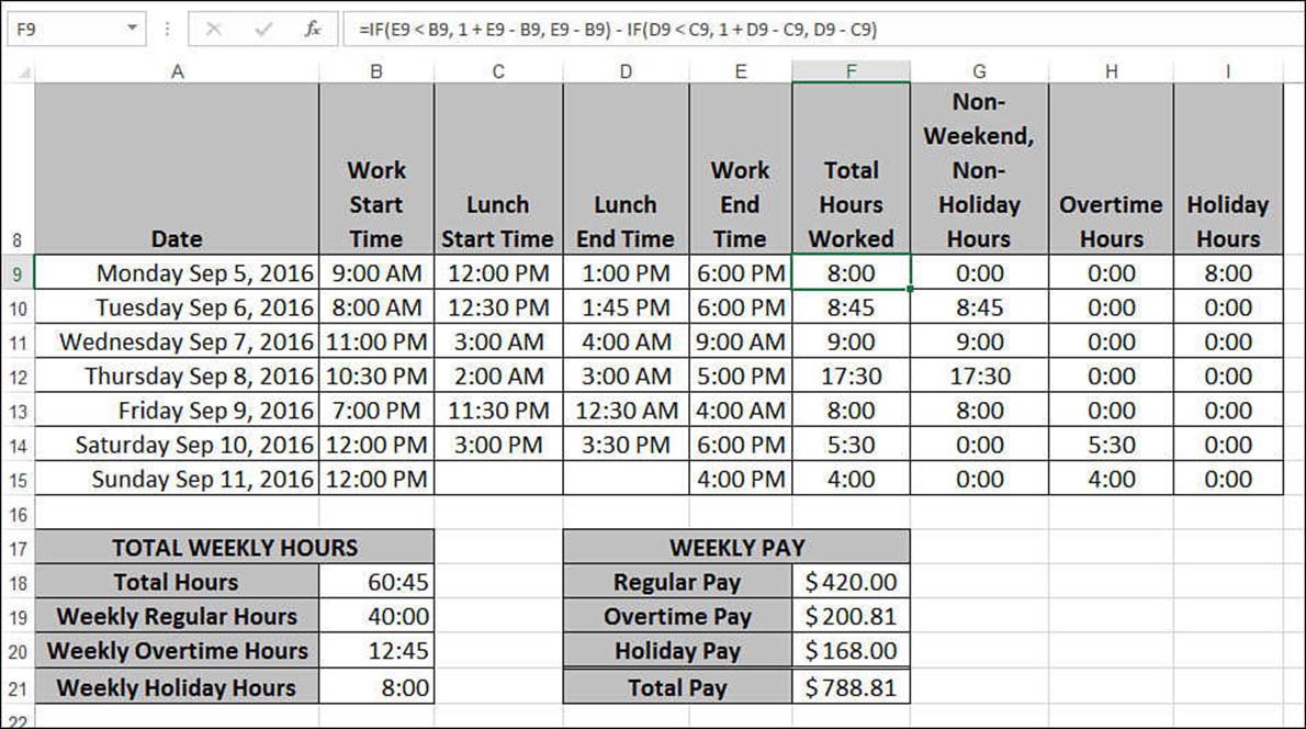
Figure 10.6 The section of the employee time sheet in which you enter the hours worked and in which the total daily hours are calculated.
The first calculation occurs in Total Hours Worked (column F). The idea here is to sum the number of hours the employee worked in a given day. The first part of the calculation uses the time-difference formula from the previous section to derive the number of hours between the Work Start Time (column B) and the Work End Time (column E). Here’s the expression for the first entry (row 9):
IF(E9 < B9, 1 + E9 - B9, E9 - B9)
However, you also have to subtract the time the employee took for lunch, which is the difference between Lunch Start Time (column C) and Lunch End Time (column D). Here’s the expression for the first entry (row 9):
IF(D9 < C9, 1 + D9 - C9, D9 - C9)
Let’s skip over to the Weekend Hours calculation (column H). The idea behind this column is that if the employee worked on the weekend, all of the hours worked should be booked as overtime hours. So, the formula checks to see whether the date is a Saturday or Sunday:
=IF(OR(WEEKDAY(A9) = 7, WEEKDAY(A9) = 1), F9, 0)
If the OR() function returns TRUE, the date is on the weekend, so the value from the Total Hours Worked column (F9, in the example) is entered into the Weekend Hours column; otherwise, 0 is returned.
Next up is the Holiday Hours calculation (column I). Here, you want to see if the date is a statutory holiday. If it is, all of the hours worked that day should be booked as holiday hours. To that end, the formula checks to see if the date is part of the range of holiday dates calculated earlier in this chapter:
{=SUM(IF(A9 = Holidays!F4:F13, 1, 0)) * F9}
This is an array formula that compares the date with the dates in the holiday range (Holidays!F4:F13). If a match occurs, the SUM() function returns 1; otherwise, it returns 0. This result is multiplied by the value in the Total Hours Worked column (F9, in the example). So, if the date is a holiday, the hours for that day are entered as holiday hours.
Finally, the value in the Non-Weekend, Non-Holiday Hours column (G) is calculated by subtracting Weekend Hours and Holiday Hours from Total Hours Worked:
=F9 - H9 - I9
Calculating the Weekly Hours Worked
Next up is the Total Weekly Hours section (refer to Figure 10.5), which adds the various types of hours the employee worked during the week.
The Total Hours value is a straight sum of the values in the Total Hours Worked column (F):
=SUM(F9:F15)
To derive the Weekly Regular Hours value, the calculation has to check to see if the total in the Non-Weekend, Non-Holiday Hours column (G) exceeds the number in the Maximum Hours Before Overtime cell (D3):
=IF(SUM(G9:G15) > D3, D3, SUM(G9:G15))
If this is true, the value in D3 is entered as the Regular Hours value; otherwise, the sum is entered.
Calculating the Weekly Overtime Hours value is a two-step process: First, you have to check to see if the sum in the Non-Weekend, Non-Holiday Hours column (G) exceeds the number in the Maximum Hours Before Overtime cell (D3). If so, the number of overtime hours is the difference between them; otherwise, it’s 0:
IF(SUM(G9:G15) > D3, SUM(G9:G15) - D3, "0:00")
Second, you need to add the sum of the Overtime Hours column (H):
=IF(SUM(G9:G15) > D3, SUM(G9:G15) - D3, "0:00") + SUM(H9:H15)
Finally, the Weekly Holiday Hours value is a straight sum of the values in the Holiday Hours column (I):
=SUM(I9:I15)
Calculating the Weekly Pay
The final section of the time sheet is the Weekly Pay calculation. The dollar amounts for Regular Pay, Overtime Pay, and Holiday Pay are calculated as follows:
Regular Pay = Weekly Regular Hours * Hourly Wage * 24
Overtime Pay = Weekly Overtime Hours * Hourly Wage * Overtime Pay Rate * 24
Holiday Pay = Weekly Holiday Hours * Hourly Wage * Holiday Pay Rate * 24
Note that you need to multiply by 24 to convert the time value to a real number. Finally, the Total Pay is the sum of these values.
From Here
![]() For more information on formatting dates and times, see “Formatting Numbers, Dates, and Times,” p. 74.
For more information on formatting dates and times, see “Formatting Numbers, Dates, and Times,” p. 74.
![]() For a general discuss of function syntax, see “The Structure of a Function,” p. 130.
For a general discuss of function syntax, see “The Structure of a Function,” p. 130.
![]() To learn how to convert nonstandard date strings to dates, see “A Date-Conversion Formula,” p. 154.
To learn how to convert nonstandard date strings to dates, see “A Date-Conversion Formula,” p. 154.
![]() To learn how to use CHOOSE() to convert the WEEKDAY() return value into a day name, see “Determining the Name of the Day of the Week,” p. 194.
To learn how to use CHOOSE() to convert the WEEKDAY() return value into a day name, see “Determining the Name of the Day of the Week,” p. 194.
All materials on the site are licensed Creative Commons Attribution-Sharealike 3.0 Unported CC BY-SA 3.0 & GNU Free Documentation License (GFDL)
If you are the copyright holder of any material contained on our site and intend to remove it, please contact our site administrator for approval.
© 2016-2026 All site design rights belong to S.Y.A.