Excel® 2016 Formulas and Functions (2016)
Part II: Harnessing the Power of Functions
11. Working with Math Functions
In This Chapter
Excel’s Math and Trig Functions
Understanding Excel’s Rounding Functions
Summing Values
The MOD() Function
Generating Random Numbers
Excel’s mathematical underpinnings are revealed in the long list of math-related functions that come with the program. Functions exist for basic mathematical operations such as absolute values, lowest and greatest common denominators, square roots, and sums. Plenty of high-end operations also are available for things such as matrix multiplication, multinomials, and sums of squares. Not all of Excel’s math functions are useful in a business context, but a surprising number of them are. For example, operations such as rounding and generating random numbers have business uses.
Excel’s Math and Trig Functions
Table 11.1 lists the Excel math functions, but this chapter doesn’t cover the entire list. Instead, I just focus on those functions that I think you’ll find useful for your business formulas. Remember, too, that Excel comes with many statistical functions, covered in Chapter 12, “Working with Statistical Functions.”
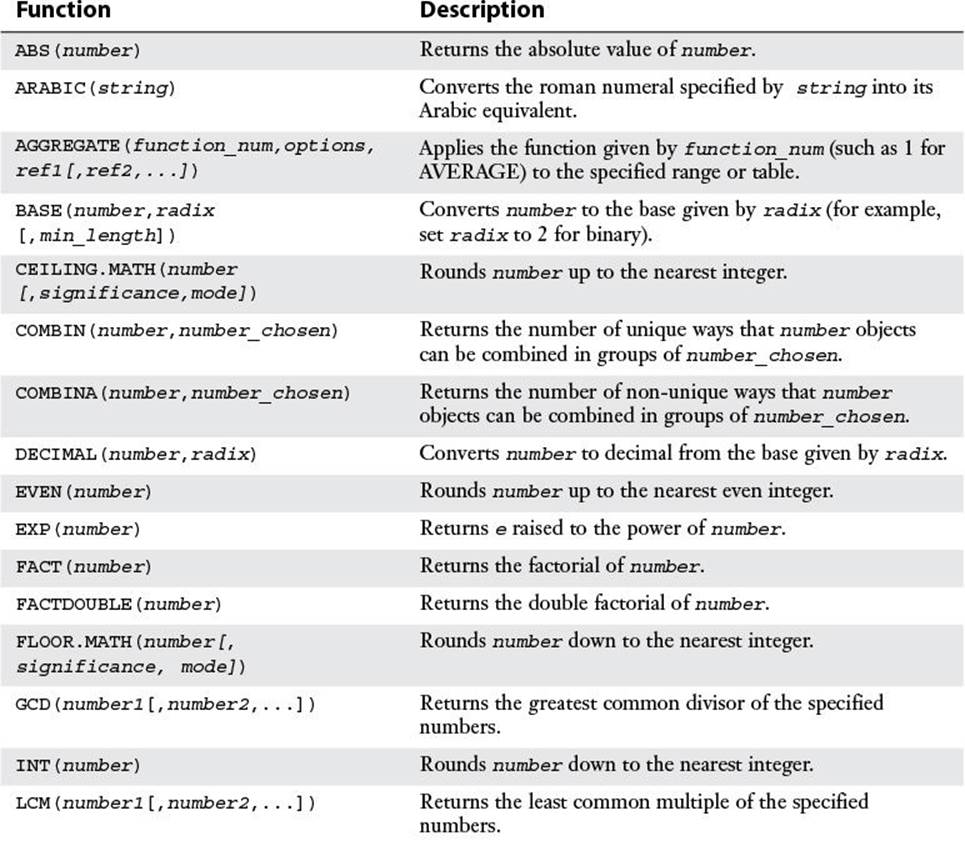
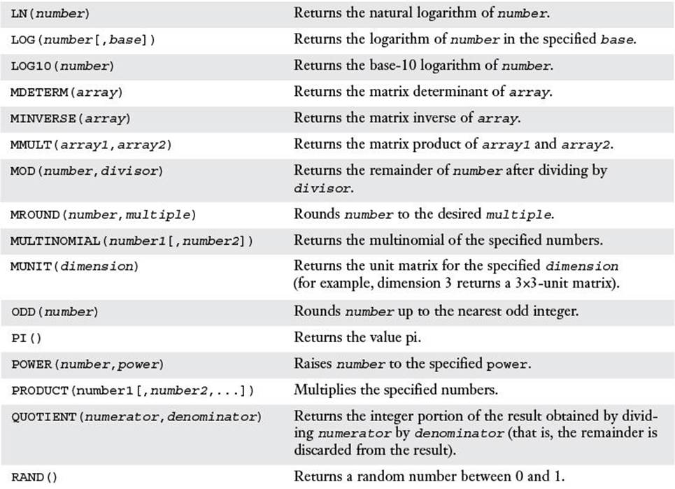
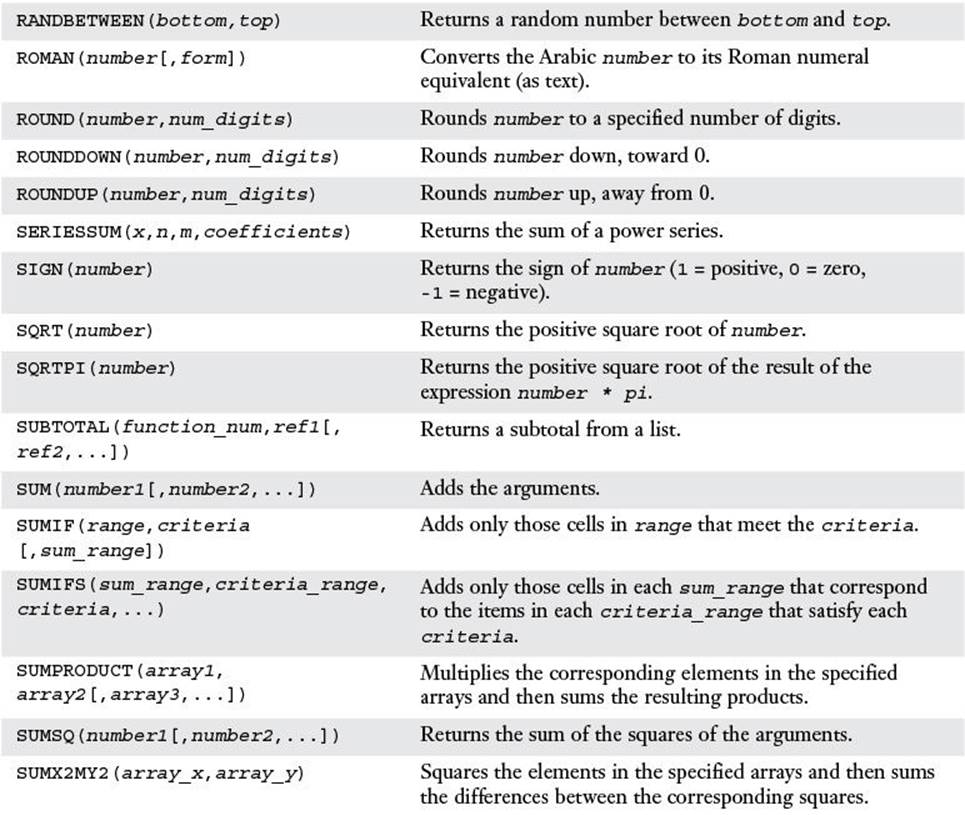
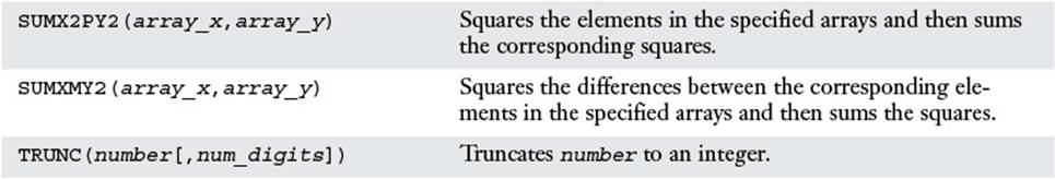
Table 11.1 Excel’s Math Functions
Although I don’t discuss the details of Excel’s trig functions in this book, Table 11.2 lists all of them. Here are some notes to keep in mind when you use these functions:
![]() In each function syntax, number is an angle expressed in radians.
In each function syntax, number is an angle expressed in radians.
![]() If you have an angle in degrees, convert it to radians by multiplying it by PI()/180. Alternatively, use the RADIANS(angle) function to convert angle from degrees to radians.
If you have an angle in degrees, convert it to radians by multiplying it by PI()/180. Alternatively, use the RADIANS(angle) function to convert angle from degrees to radians.
![]() A trig function returns a value in radians. If you need to convert a result to degrees, multiply it by 180/PI(). Alternatively, use the DEGREES(angle) function, which converts angle from radians to degrees.
A trig function returns a value in radians. If you need to convert a result to degrees, multiply it by 180/PI(). Alternatively, use the DEGREES(angle) function, which converts angle from radians to degrees.
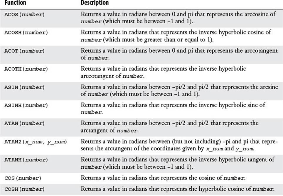
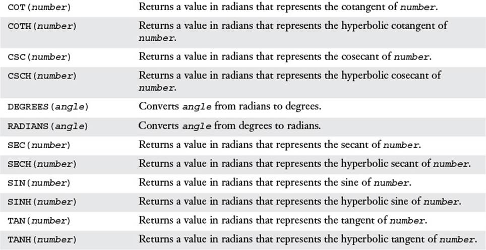
Table 11.2 Excel’s Trigonometric Functions
Understanding Excel’s Rounding Functions
Excel’s rounding functions are useful in many situations, such as setting price points, adjusting billable time to the nearest 15 minutes, and ensuring that you’re dealing with integer values for discrete numbers, such as inventory counts.
The problem is that Excel has so many rounding functions that it’s difficult to know which one to use in a given situation. To help you, this section looks at the details of—and differences between—Excel’s 10 rounding functions: ROUND(), MROUND(), ROUNDUP(), ROUNDDOWN(),CEILING.MATH(), FLOOR.MATH(), EVEN(), ODD(), INT(), and TRUNC().
The ROUND() Function
The rounding function you’ll use most often is ROUND():
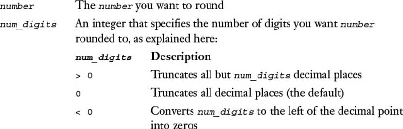
ROUND(number, num_digits)
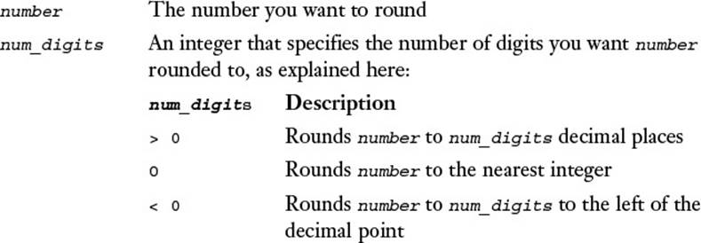
Table 11.3 demonstrates the effect of the num_digits argument on the results of the ROUND() function. Here, number is 1234.5678.
Table 11.3 Effect of the num_digits Argument on the ROUND() Function Result
The MROUND() Function
MROUND() is a function that rounds a number to a specified multiple:
MROUND(number, multiple)

Table 11.4 demonstrates MROUND() with a few examples. Note that if number and multiple have different signs, MROUND() produces the #NUM! error.
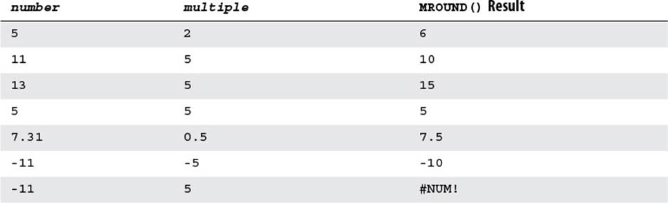
Table 11.4 Examples of the MROUND() Function
The ROUNDDOWN() and ROUNDUP() Functions
The ROUNDDOWN() and ROUNDUP() functions are similar to ROUND(), except that they always round in a single direction: ROUNDDOWN() always rounds a number toward 0, and ROUNDUP() always rounds away from 0. Here is the syntax for each of these functions:
ROUNDDOWN(number, num_digits)
ROUNDUP(number, num_digits)
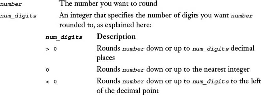
Table 11.5 tries out ROUNDDOWN() and ROUNDUP() with a few examples.
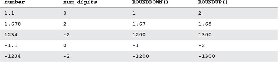
Table 11.5 Examples of the ROUNDDOWN() and ROUNDUP() Functions
The CEILING.MATH() and FLOOR.MATH() Functions
The CEILING.MATH() and FLOOR.MATH() functions are an amalgam of the features found in MROUND(), ROUNDDOWN(), and ROUNDUP(). Here is the syntax of each one:
CEILING.MATH(number[, significance, mode])
FLOOR.MATH(number[, significance, mode])
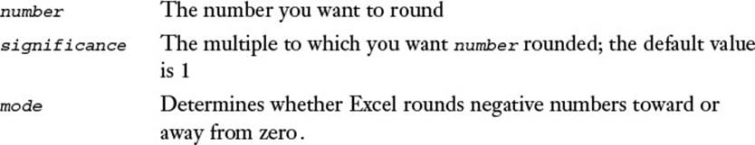
Both functions round the value given by number to a multiple of the value given by significance, but they differ in how they perform this rounding:
![]() CEILING.MATH() rounds positive numbers away from 0 and negative numbers toward 0. For example, CEILING.MATH(1.56, 0.1) returns 1.6, and CEILING.MATH(-2.33, 0.5) returns -2. If you prefer to round negative numbers away from 0, add the modeparameter with any nonzero value.
CEILING.MATH() rounds positive numbers away from 0 and negative numbers toward 0. For example, CEILING.MATH(1.56, 0.1) returns 1.6, and CEILING.MATH(-2.33, 0.5) returns -2. If you prefer to round negative numbers away from 0, add the modeparameter with any nonzero value.
![]() FLOOR.MATH() rounds positive numbers toward 0 and negative numbers away from 0. For example, FLOOR.MATH(1.56, 0.1) returns 1.5, and FLOOR.MATH(-2.33, -.5) returns -2.35. If you prefer to round negative numbers toward 0, add the mode parameter with any nonzero value.
FLOOR.MATH() rounds positive numbers toward 0 and negative numbers away from 0. For example, FLOOR.MATH(1.56, 0.1) returns 1.5, and FLOOR.MATH(-2.33, -.5) returns -2.35. If you prefer to round negative numbers toward 0, add the mode parameter with any nonzero value.
Determining the Fiscal Quarter in Which a Date Falls
When working with budget-related or other financial worksheets, you often need to know the fiscal quarter in which a particular date falls. For example, a budget increase formula might need to alter the increase depending on the quarter.
You can use the CEILING.MATH() function combined with the DATEDIF() function from Chapter 10, “Working with Date and Time Functions,” to calculate the quarter for a given date:
=CEILING.MATH((DATEDIF(FiscalStart, MyDate, "m") + 1) / 3, 1)
![]() To learn about DATEDIF(), see “The DATEDIF() Function,” p. 224.
To learn about DATEDIF(), see “The DATEDIF() Function,” p. 224.
Here, FiscalStart is the date on which the fiscal year begins, and MyDate is the date you want to work with. This formula uses DATEDIF() with the m parameter to return the number of months between the two dates. The formula adds 1 to the result (to avoid getting a 0th quarter) and then divides by 3. Applying CEILING.MATH() to the result gives the quarter in which MyDate occurs.
Calculating Easter Dates
If you live or work in the United States, you’ll rarely have to calculate for business purposes when Easter Sunday falls because there’s no statutory holiday associated with Easter. However, if Good Friday or Easter Monday is a statutory holiday where you live (as Good Friday is in Canada and Easter Monday is in Britain), or if you’re responsible for businesses in such jurisdictions, it can be handy to calculate when Easter falls in a given year.
Unfortunately, there’s no straightforward way of calculating Easter. The official formula is that Easter falls on the first Sunday after the first ecclesiastical full moon after the spring equinox. Mathematicians have tried for centuries to come up with a formula, and although some have succeeded (most notably the famous mathematician Carl Friedrich Gauss), the resulting algorithms have been hideously complex.
Here’s a relatively simple worksheet formula that employs the FLOOR.MATH() function and that works for the years 1900 to 2078:
=FLOOR.MATH(DATE(B1, 5, DAY(MINUTE(B1 / 38) / 2 + 56)), 7) - 36
This formula assumes that the current year is in cell B1.
![]() To learn how to calculate when Good Friday and Easter Monday fall, see “Calculating Holiday Dates,” p. 221.
To learn how to calculate when Good Friday and Easter Monday fall, see “Calculating Holiday Dates,” p. 221.
The EVEN() and ODD() Functions
The EVEN() and ODD() functions round a single numeric argument:
EVEN(number)
ODD(number)
![]()
Both functions round the value given by number away from 0, as follows:
![]() EVEN() rounds to the next even number. For example, EVEN(14.2) returns 16, and EVEN(-23) returns -24.
EVEN() rounds to the next even number. For example, EVEN(14.2) returns 16, and EVEN(-23) returns -24.
![]() ODD() rounds to the next odd number. For example, ODD(58.1) returns 59 and ODD(-6) returns -7.
ODD() rounds to the next odd number. For example, ODD(58.1) returns 59 and ODD(-6) returns -7.
The INT() and TRUNC() Functions
The INT() and TRUNC() functions are similar in that you can use both of them to convert a value to its integer portion:
INT(number)
TRUNC(number[, num_digits])
For example, INT(6.75) returns 6, and TRUNC(3.6) returns 3. However, these functions have two major differences that you should keep in mind:
![]() For negative values, INT() returns the next number away from 0. For example, INT(-3.42) returns -4. If you just want to lop off the decimal part, you need to use TRUNC() instead.
For negative values, INT() returns the next number away from 0. For example, INT(-3.42) returns -4. If you just want to lop off the decimal part, you need to use TRUNC() instead.
![]() You can use the TRUNC() function’s second argument (num_digits) to specify the number of decimal places to leave on. For example, TRUNC(123.456, 2) returns 123.45, and TRUNC(123.456, -2) returns 100.
You can use the TRUNC() function’s second argument (num_digits) to specify the number of decimal places to leave on. For example, TRUNC(123.456, 2) returns 123.45, and TRUNC(123.456, -2) returns 100.
Using Rounding to Prevent Calculation Errors
Most of us are comfortable dealing with numbers in decimal—or base-10—format (the odd hexadecimal-loving computer geek notwithstanding). Computers, however, prefer to work in the simpler confines of the binary—or base-2—system. So when you plug a value into a cell or formula, Excel converts it from decimal to its binary equivalent, makes its calculations, and then converts the binary result back into decimal format.
This procedure is fine for integers because every decimal integer value has an exact binary equivalent. However, many noninteger values don’t have exact equivalents in the binary world. Excel can only approximate such numbers, and that approximation can lead to errors in formulas. For example, try entering the following formula into any worksheet cell:
=0.01 = (2.02 - 2.01)
This formula compares the value 0.01 with the expression 2.02 - 2.01. These should be equal, of course, but when you enter the formula, Excel returns a FALSE result. What gives?
The problem is that, in converting the expression 2.02 - 2.01 into binary and back again, Excel picks up a stray digit in its travels. To see it, enter the formula =2.02 - 2.01 in a cell and then format it to show 16 decimal places. You should see the following surprising result:
0.0100000000000002
That wanton 2 in the 16th decimal place is what threw off the original calculation. To fix the problem, use the TRUNC() function (or possibly the ROUND() function, depending on the situation) to lop off the extra digits to the right of the decimal point. For example, the following formula produces a TRUE result:
=0.01 = TRUNC(2.02 - 2.01, 2)
Setting Price Points
One common worksheet task is to calculate a list price for a product based on the result of a formula that factors in production costs and profit margin. If the product will be sold at retail, you’ll likely want the decimal (cents) portion of the price to be .95, .99, or some other standard value. You can use the INT() function to help with this “rounding.”
For example, the simplest case is to always round up the decimal part to .95. Here’s a formula that does this:
=INT(RawPrice) + 0.95
Assuming that RawPrice is the result of the formula that factors in costs and profit, the formula simply adds 0.95 to the integer portion. (Note, too, that if the decimal portion of RawPrice is greater than .95, the formula rounds down to .95.)
Another case is to round up to .50 for decimal portions less than or equal to 0.5 and to round up to .95 for decimal portions greater than 0.5. Here’s a formula that handles this scenario:
=INT(RawPrice) + IF(RawPrice - INT(RawPrice) <= 0.5, .50, .95)
Again, the integer portion is stripped from the RawPrice. Also, the IF() function checks to see whether the decimal portion is less than or equal to 0.5. If it is, the value .50 is returned; otherwise, the value .95 is returned. This result is added to the integer portion.
Case Study: Rounding Billable Time
An ideal use of MROUND() is to round billable time to some multiple number of minutes. For example, it’s common to round billable time to the nearest 15 minutes. You can do this with MROUND() by using the following generic form of the function:
MROUND(BillableTime, 0:15)
Here, BillableTime is the time value you want to round. For example, the following expression returns the time value 2:15:
MROUND(2:10, 0:15)
Using MROUND() to round billable time has one significant flaw: Many (perhaps even most) people who bill their time prefer to round up to the nearest 15 minutes (or whatever). If the minute component of the MROUND() function’s number argument is less than half the multipleargument, MROUND() rounds down to the nearest multiple.
To fix this problem, use the CEILING.MATH() function instead because it always rounds away from 0. Note, however, that CEILING.MATH() will only work in this scenario if you express your times using the TIME() function. Here’s the generic expression to use for rounding up to the next 15-minute multiple:
CEILING.MATH(TIME(BillableHours,BillableMinutes,BillableSeconds,)
TIME(0,15,0))
Here, BillableHours, BillableMinutes, and BillableSeconds are the components of the time value you want to round. For example, the following expression rounds the time value 2:05 up to the time value 2:15:
CEILING.MATH(TIME(2, 5, 0), TIME(0, 15, 0))
Summing Values
Summing values—whether it’s a range of cells, function results, literal numeric values, or expression results—is perhaps the most common spreadsheet operation. Excel enables you to add values by using the addition operator (+), but it’s often more convenient to sum a number of values by using the SUM() function, which you’ll learn more about in the next section.
The SUM() Function
Here’s the syntax of the SUM() function:
SUM(number1[, number2, ...])
![]()
In Excel 2007 and later, you can enter up to 255 arguments into the SUM() function. (In previous versions of Excel, the maximum number of arguments is 30.) Note, too, that you can enter the SUM() quickly by clicking the AutoSum command that appears in both the Home tab and the Formulas tab (or by pressing Alt+=).
For example, the following formula returns the sum of the values in three separate ranges:
=SUM(A2:A13, C2:C13, E2:E13)
Tip
If you need more than 255 arguments for the SUM() function, group multiple arguments together using parentheses. For example, SUM(A1, B1, C1, D1) uses four arguments, but Excel sees SUM((A1, B1), (C1, D1)) as using just two arguments.
Calculating Cumulative Totals
Many worksheets need to calculate cumulative totals. Most budget worksheets, for example, show cumulative totals for sales and expenses over the course of the fiscal year. Similarly, loan amortizations often show the cumulative interest and principal paid over the life of the loan.
Calculating these cumulative totals is straightforward. For example, see the worksheet shown in Figure 11.1. Column F tracks the cumulative interest on the loan, and cell F7 contains the following SUM() formula:
=SUM($D$7:D7)
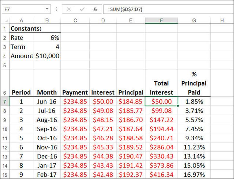
Figure 11.1 The SUM() formulas in column F calculate the cumulative interest paid on a loan.
Note
You can download this chapter’s sample workbook at www.mcfedries.com/books/book.php?title=excel-2016-formulas-and-functions.
This formula just sums cell D7, which is no great feat. However, when you fill the range F7:F54 with this formula, the left part of the SUM() range ($D$7) remains anchored; the right side (D7) is relative and, therefore, changes. So, for example, the corresponding formula in cell F10 would be this:
=SUM($D$7:D10)
In case you’re wondering, column G tracks the percentage of the total principal that has been paid off so far. Here’s the formula used in cell G7:
=SUM($E$7:E7) / $B$4 * -1
The SUM($E$7:E7) part calculates the cumulative principal paid. To get the percentage, divide by the total principal (cell B4). The whole thing is multiplied by −1 to return a positive percentage.
Summing Only the Positive or Negative Values in a Range
If you have a range of numbers that contains both positive and negative values, what do you do if you need a total of only the negative values? Or only the positive ones? You could enter the individual cells into a SUM() function, but there’s an easier way: use arrays.
To sum the negative values in a range, you use the following array formula:
{=SUM((range < 0) * range)}
Here, range is a range reference or named range. The range < 0 test returns TRUE (the equivalent of 1) for those range values that are less than 0; otherwise, it returns FALSE (the equivalent of 0). Therefore, only negative values get included in the SUM().
Similarly, you use the following array formula to sum only the positive values in range:
{=SUM((range > 0) * range)}
![]() You can apply much more sophisticated criteria to your sums by using the SUMIF() function. See “Using SUMIF(),” p. 314.
You can apply much more sophisticated criteria to your sums by using the SUMIF() function. See “Using SUMIF(),” p. 314.
The MOD() Function
The MOD() function calculates the remainder (or modulus) that results after dividing one number into another. Here’s the syntax for this more-useful-than-you-think function:
MOD(number, divisor)
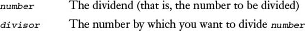
For example, MOD(24, 10) equals 4 (that is, 24÷10 = 2, with remainder 4).
The MOD() function is well suited to values that are both sequential and cyclical. For example, the days of the week (as given by the WEEKDAY() function) run from 1 (Sunday) through 7 (Saturday) and then start over (the next Sunday is back to 1). So, the following formula always returns an integer that corresponds to a day of the week:
=MOD(number, 7) + 1
If number is any integer, the MOD() function returns integer values from 0 to 6, so adding 1 gives values from 1 to 7.
You can set up similar formulas using months (1 to 12), seconds or minutes (0 to 59), fiscal quarters (1 to 4), and more.
A Better Formula for Time Differences
In Chapter 10, I told you that subtracting an earlier time from a later time is problematic if the earlier time is before midnight and the later time is after midnight. Here’s the expression I showed you to overcome this problem:
IF(EndTime < StartTime, 1 + EndTime - StartTime, EndTime - StartTime)
![]() For the details on the time-difference formula, see “Calculating the Difference Between Two Times,” p. 231.
For the details on the time-difference formula, see “Calculating the Difference Between Two Times,” p. 231.
However, time values are sequential and cyclical: They’re real numbers that run from 0 to 1 and then start over at midnight. Therefore, you can use MOD() to greatly simplify the formula for calculating the difference between two times:
=MOD(EndTime - StartTime, 1)
This works for any value of EndTime and StartTime, as long as EndTime is later than StartTime.
Summing Every nth Row
Depending on the structure of your worksheet, you might need to sum only every nth row, where n is some integer. For example, you might want to sum only every 5th or 10th cell to get a sampling of the data.
You can accomplish this by applying the MOD() function to the result of the ROW() function, as in this array formula:
{=SUM(IF(MOD(ROW(Range), n) = 1, Range, 0))}
For each cell in Range, MOD(ROW(Range), n) returns 1 for every nth value. In that case, the value of the cell is added to the sum; otherwise, 0 is added. In other words, this sums the values in the first row of Range, the n + first row of Range, and so on. If instead you want the second row of Range, the n + second row of Range, and so on, compare the MOD() result with 2, like so:
{=SUM(IF(MOD(ROW(Range), n) = 2, Range, 0))}
Special Case No. 1: Summing Only Odd Rows
If you want to sum only the odd rows in a worksheet, use this straightforward variation on the formula:
{=SUM(IF(MOD(ROW(Range), 2) = 1, Range, 0))}
Special Case No. 2: Summing Only Even Rows
To sum only the even rows, you need to sum those cells where MOD(ROW(Range), 2) returns 0:
{=SUM(IF(MOD(ROW(Range), 2) = 0, Range, 0))}
Determining Whether a Year Is a Leap Year
If you need to determine whether a given year is a leap year, the MOD() function can help. Leap years (with some exceptions) are years divisible by 4. So, a year is (usually) a leap year if the following formula returns 0:
=MOD(year, 4)
In this case, year is a four-digit year number. This formula works for the years 1901 to 2099, which should take care of most people’s needs. The formula doesn’t work for 1900 and 2100 because, despite being divisible by 4, these years aren’t leap years. The general rule is that a year is a leap year if it’s divisible by 4 and it’s not divisible by 100, unless it’s also divisible by 400. Therefore, because 1900 and 2100 are divisible by 100 and not by 400, they aren’t leap years. The year 2000, however, is a leap year. If you want a formula that takes the full rule into account, use the following one:
=(MOD(year, 4) = 0) - (MOD(year, 100) = 0) + (MOD(year, 400) = 0)
The three parts of the formula that compare a MOD() result to 0 return 1 or 0. Therefore, the result of this formula always is 0 for leap years and nonzero for all other years.
Creating Ledger Shading
Ledger shading is formatting in which rows alternate cell shading between a light color and a slightly darker color (for example, white and light gray). This type of shading is often seen in checkbook registers and account ledgers, but it’s also useful in any worksheet that presents data in rows because it makes differentiating each row from its neighbors easier. Figure 11.2 shows an example.
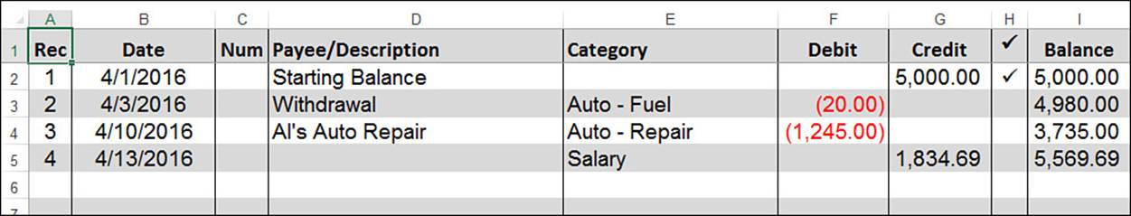
Figure 11.2 This worksheet uses ledger shading for a checkbook register.
However, ledger shading isn’t easy to work with by hand:
![]() If you have a large range to format, applying shading can take some time.
If you have a large range to format, applying shading can take some time.
![]() If you insert or delete a row, you have to reapply the formatting.
If you insert or delete a row, you have to reapply the formatting.
To avoid these headaches, you can use a trick that combines the MOD() function and Excel’s conditional formatting. Here’s how it’s done:
1. Select the area you want to format with ledger shading.
2. Select Home, Conditional Formatting, New Rule to display the New Formatting Rule dialog box.
3. Click Use a Formula to Determine Which Cells to Format.
4. In the text box, enter the following formula:
=MOD(ROW(), 2)
5. Click Format to display the Format Cells dialog box.
6. Select the Fill tab, click the color you want to use for the nonwhite ledger cells, and then click OK to return to the New Formatting Rule dialog box (see Figure 11.3).
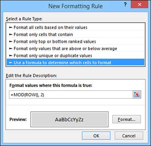
Figure 11.3 This MOD() formula applies the cell shading to every second row (1, 3, 5, and so on).
7. Click OK.
The formula =MOD(ROW(), 2) returns 1 for odd-numbered rows and 0 for even-numbered rows. Because 1 is equivalent to TRUE, Excel applies the conditional formatting to the odd-numbered rows and leaves the even-numbered rows as they are.
Tip
If you prefer to alternate shading on columns instead of on rows, use the following formula in the New Formatting Rule dialog box:
=MOD(COLUMN(), 2)
If you prefer to have the even rows shaded and the odd rows unshaded, use the following formula in the New Formatting Rule dialog box:
=MOD(ROW() + 1, 2)
Generating Random Numbers
If you’re using a worksheet to set up a simulation, you need realistic data on which to do your testing. You could make up the numbers, but it’s possible that you might unintentionally skew the data. A better approach is to generate the numbers randomly, using the worksheet functionsRAND() and RANDBETWEEN().
![]() Excel’s Analysis ToolPak also comes with a tool for generating random numbers; see “Using the Random Number Generation Tool,” p. 285.
Excel’s Analysis ToolPak also comes with a tool for generating random numbers; see “Using the Random Number Generation Tool,” p. 285.
The RAND() Function
The RAND() function returns a random number that is greater than or equal to 0 and less than 1. RAND() is often useful by itself. (For example, it’s perfect for generating random time values.) However, you’ll most often use it in an expression to generate random numbers between two values.
In the simplest case, if you want to generate random numbers greater than or equal to 0 and less than n, use the following expression:
RAND() * n
For example, the following formula generates a random number between 0 and 30:
=RAND() * 30
The more complex case is when you want random numbers greater than or equal to some number m and less than some number n. Here’s the expression to use for this case:
RAND() * (n - m) + m
For example, the following formula produces a random number greater than or equal to 100 and less than 200:
=RAND() * (200 - 100) + 100
Caution
RAND() is a volatile function, meaning that its value changes each time you recalculate or reopen the worksheet or edit any cell on the worksheet. To enter a static random number in a cell, type =RAND(), press F9 to evaluate the function and return a random number, and then press Enter to place the random number into the cell as a numeric literal.
Generating Random n-Digit Numbers
It’s often useful to create random numbers with a specific number of digits. For example, you might want to generate a random six-digit account number for new customers, or you might need a random eight-digit number for a temporary filename.
The procedure for this is to start with the general formula from the previous section and apply the INT() function to ensure an integer result:
INT(RAND() * (n - m) + m)
In this case, however, you set n equal to 10n, and you set m equal to 10n-1:
INT(RAND() * (10n - 10n-1) + 10n-1)
For example, if you need a random eight-digit number, use this formula:
INT(RAND() * (100000000 - 10000000) + 10000000)
This generates random numbers greater than or equal to 10,000,000 and less than or equal to 99,999,999.
Generating a Random Letter
You normally use RAND() to generate a random number, but it’s also useful for text values. For example, suppose that you need to generate a random letter of the alphabet. There are 26 letters in the alphabet, so you start with an expression that generates random integers greater than or equal to 1 and less than or equal to 26:
INT(RAND() * 26 + 1)
If you want a random uppercase letter (A to Z), note that these letters have character codes that run from ANSI 65 to ANSI 90, so you take the preceding formula, add 64, and plug in the result to the CHAR() function:
=CHAR(INT(RAND() * 26) + 65)
If you want a random lowercase letter (a to z) instead, note that these letters have character codes that run from ANSI 97 to ANSI 122, so you take the preceding formula, add 96, and plug the result into the CHAR() function:
=CHAR(INT(RAND() * 26) + 97)
Sorting Values Randomly
If you have a set of values on a worksheet, you might need to sort them in random order. For example, if you want to perform an operation on a subset of data, sorting the table randomly removes any numeric biases that might be inherent if the data was sorted in any way.
Follow these steps to randomly sort a data table:
1. Assuming that the data is arranged in rows, select a range in the column immediately to the left or right of the table. Make sure that the selected range has the same number of rows as the table.
2. Enter =RAND() and then press Ctrl+Enter to add the RAND() formula to every selected cell.
3. Select Formulas, Calculation Options, Manual.
4. Select the range that includes the data and the column of RAND() values.
5. Select Data, Sort to display the Sort dialog box.
6. In the Sort By list, select the column that contains the RAND() values.
7. Click OK.
8. Select Formulas, Calculation Options, Automatic and delete the RAND() formulas from the table.
This procedure tells Excel to sort the selected range according to the random values, thus sorting the data table randomly. Figure 11.4 shows an example. The data values are in column A, the RAND() values are in column B, and the range A2:B26 was sorted on column B.
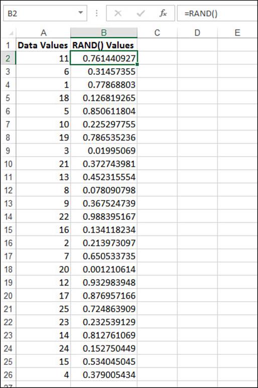
Figure 11.4 To randomly sort data values, add a column of =RAND() formulas and then sort the entire range on the random values.
The RANDBETWEEN() Function
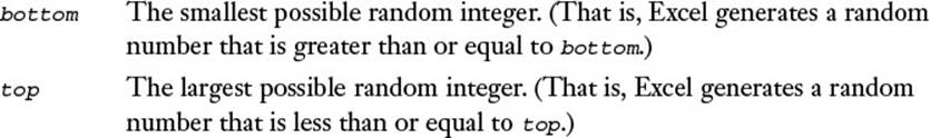
Excel’s RANDBETWEEN() function can simplify working with certain sets of random numbers. RANDBETWEEN() lets you specify a lower bound and an upper bound, and it returns a random integer between them:
RANDBETWEEN(bottom, top)
For example, the following formula returns a random integer between 0 and 59:
=RANDBETWEEN(0, 59)
From Here
![]() Excel comes with a large collection of statistical functions for calculating averages, maximums and minimums, standard deviations, and more. See Chapter 12, “Working with Statistical Functions,” p. 257.
Excel comes with a large collection of statistical functions for calculating averages, maximums and minimums, standard deviations, and more. See Chapter 12, “Working with Statistical Functions,” p. 257.
![]() To learn how to create sophisticated distributions of random numbers, see “Using the Random Number Generation Tool,” p. 285.
To learn how to create sophisticated distributions of random numbers, see “Using the Random Number Generation Tool,” p. 285.
![]() The SUMIF() function enables you to apply sophisticated criteria to sum operations. See “Using SUMIF(),” p. 314.
The SUMIF() function enables you to apply sophisticated criteria to sum operations. See “Using SUMIF(),” p. 314.
All materials on the site are licensed Creative Commons Attribution-Sharealike 3.0 Unported CC BY-SA 3.0 & GNU Free Documentation License (GFDL)
If you are the copyright holder of any material contained on our site and intend to remove it, please contact our site administrator for approval.
© 2016-2026 All site design rights belong to S.Y.A.