Excel® 2016 Formulas and Functions (2016)
Part III: Building Business Models
13. Analyzing Data with Tables
In This Chapter
Planning an Excel Table
Converting a Range to a Table
Basic Table Operations
Sorting a Table
Filtering Table Data
Referencing Tables in Formulas
Excel’s Table Functions
Excel’s forte is spreadsheet work, of course, but its row-and-column layout also makes it a natural flat-file database manager. In Excel, a table is a collection of related information with an organizational structure that makes it easy to find or extract data from its contents. (In legacy versions of Excel—that is, in versions prior to Excel 2007—a table was called a list.) Specifically, a table is a worksheet range that has the following properties:
![]() Field—A single type of information, such as a name, an address, or a phone number. In Excel tables, each column is a field.
Field—A single type of information, such as a name, an address, or a phone number. In Excel tables, each column is a field.
![]() Field name—A unique name you assign to every table field. These names are always found in the first row of the table.
Field name—A unique name you assign to every table field. These names are always found in the first row of the table.
![]() Field value—A single item in a field. In an Excel table, the field values are the individual cells.
Field value—A single item in a field. In an Excel table, the field values are the individual cells.
![]() Record—A collection of associated field values. In Excel tables, each row is a record.
Record—A collection of associated field values. In Excel tables, each row is a record.
![]() Table range—The worksheet range that includes all the records, fields, and field names of a table.
Table range—The worksheet range that includes all the records, fields, and field names of a table.
Planning an Excel Table
Suppose you want to set up an accounts receivable table. A simple system would include information such as the account name, account number, invoice number, invoice amount, due date, and date paid, as well as a calculation of the number of days overdue. Figure 13.1 shows how this system would be implemented as an Excel range.
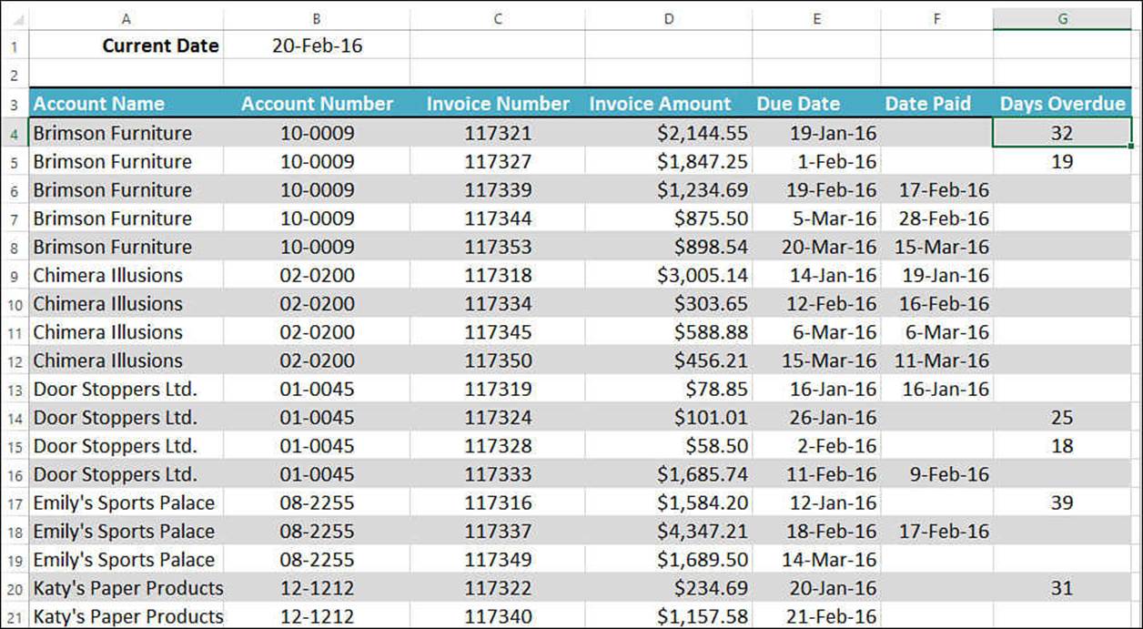
Figure 13.1 Accounts receivable data in an Excel worksheet.
Note
You can download this chapter’s sample workbook at www.mcfedries.com/books/book.php?title=excel-2016-formulas-and-functions.
Excel tables don’t require elaborate planning, but you should follow a few guidelines for best results. Here are some pointers:
![]() Always use the top row of a table for the column labels.
Always use the top row of a table for the column labels.
![]() Field names must be unique, and they must be text or text formulas. If you need to use numbers, format them as text.
Field names must be unique, and they must be text or text formulas. If you need to use numbers, format them as text.
![]() Some Excel commands can automatically identify the size and shape of a table. To avoid confusing such commands, try to use only one table per worksheet. If you have multiple related tables, include them in other worksheets in the same workbook.
Some Excel commands can automatically identify the size and shape of a table. To avoid confusing such commands, try to use only one table per worksheet. If you have multiple related tables, include them in other worksheets in the same workbook.
![]() If you have nontable data in the same worksheet, leave at least one blank row or column between the data and the table. This helps Excel identify the table automatically.
If you have nontable data in the same worksheet, leave at least one blank row or column between the data and the table. This helps Excel identify the table automatically.
![]() Excel has a command that enables you to filter your table data to show only records that match certain criteria. (See “Filtering Table Data,” later in this chapter, for details.) This command works by hiding rows of data. Therefore, if the same worksheet contains nontable data that you need to see or work with, don’t place this data to the left or right of the table.
Excel has a command that enables you to filter your table data to show only records that match certain criteria. (See “Filtering Table Data,” later in this chapter, for details.) This command works by hiding rows of data. Therefore, if the same worksheet contains nontable data that you need to see or work with, don’t place this data to the left or right of the table.
Converting a Range to a Table
Excel has a number of commands that enable you to work efficiently with table data. To take advantage of these commands, you must convert your data from a normal range to a table. Here are the steps to follow:
1. Click any cell within the range that you want to convert to a table.
2. You now have two choices:
• To create a table with the default formatting, select Insert, Table (or press Ctrl+T).
• To create a table with the formatting you specify, select Home, Format as Table and then click a table style in the gallery that appears.
Excel displays the Create Table dialog box (or the Format as Table dialog box).
3. Ensure that the Where Is the Data for Your Table? box already shows the correct range coordinates. If it doesn’t, enter the range coordinates or select the range directly on the worksheet.
4. If your range has column headers in the top row (as it should), make sure the My Table Has Headers check box is selected.
5. Click OK.
When you convert a range to a table, Excel makes three changes to the range, as shown in Figure 13.2:
![]() It formats the table cells.
It formats the table cells.
![]() It adds drop-down arrows to each field header.
It adds drop-down arrows to each field header.
![]() In the Ribbon, you see a new Design tab under Table Tools whenever you select a cell within the table.
In the Ribbon, you see a new Design tab under Table Tools whenever you select a cell within the table.
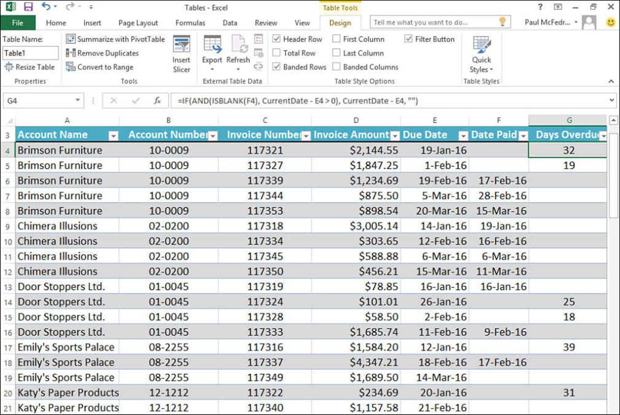
Figure 13.2 The accounts receivable data converted to a table.
Note
If you ever need to change a table back to a range, select a cell within the table and select Design, Convert to Range.
Basic Table Operations
After you’ve converted a range to a table, you can start working with the data. Here’s a quick look at some basic table operations:
![]() Selecting a record—Move the mouse pointer to the left edge of the leftmost column in the row you want to select (the pointer changes to a right-pointing arrow) and then click. You can also select any cell in the record and then press Shift+Spacebar.
Selecting a record—Move the mouse pointer to the left edge of the leftmost column in the row you want to select (the pointer changes to a right-pointing arrow) and then click. You can also select any cell in the record and then press Shift+Spacebar.
![]() Selecting a field—Move the mouse pointer to the top edge of the column header. (The pointer changes to a downward-pointing arrow.) Click once to select just the field’s data; click a second time to add the field’s header to the selection. You can also select any cell in the field and then press Ctrl+Spacebar to select the field data; press Ctrl+Spacebar again to add the header to the selection.
Selecting a field—Move the mouse pointer to the top edge of the column header. (The pointer changes to a downward-pointing arrow.) Click once to select just the field’s data; click a second time to add the field’s header to the selection. You can also select any cell in the field and then press Ctrl+Spacebar to select the field data; press Ctrl+Spacebar again to add the header to the selection.
![]() Selecting an entire table—Move the mouse pointer to the upper-left corner of a table (the pointer changes to an arrow pointing down and to the right) and then click. You can also select any cell in the table and press Ctrl+A.
Selecting an entire table—Move the mouse pointer to the upper-left corner of a table (the pointer changes to an arrow pointing down and to the right) and then click. You can also select any cell in the table and press Ctrl+A.
![]() Adding a new record at the bottom of a table—Select any cell in the row below a table, type the data you want to add to the cell, and press Enter. Excel’s AutoExpansion feature expands the table to include the new row. This also works if you select the last cell in the last row of the table and then press Tab.
Adding a new record at the bottom of a table—Select any cell in the row below a table, type the data you want to add to the cell, and press Enter. Excel’s AutoExpansion feature expands the table to include the new row. This also works if you select the last cell in the last row of the table and then press Tab.
Note
In legacy versions of Excel, you could work with table (list) records using a data form, a dialog box that enabled you to add, edit, delete, and find table records quickly. The Form command didn’t make it into Excel’s Ribbon interface, but it still exists. If you prefer using a data form to work with a table, add the Form command to the Quick Access Toolbar. Pull down the Customize Quick Access Toolbar menu and click More Commands. In the Choose Commands From list, select All Commands and then click Form in the command list. Click Add and then click OK.
![]() Adding a new record anywhere in a table—Select any cell in a record below which you want to add a new record. In the Home tab, select Insert, Insert Table Rows Above. Excel inserts a blank row above the selected cell into which you can enter the new data.
Adding a new record anywhere in a table—Select any cell in a record below which you want to add a new record. In the Home tab, select Insert, Insert Table Rows Above. Excel inserts a blank row above the selected cell into which you can enter the new data.
![]() Adding a new field to the right of a table—Select any cell in the column to the right of a table, type the data you want to add to the cell, and press Enter. AutoExpansion expands the table to include the new field.
Adding a new field to the right of a table—Select any cell in the column to the right of a table, type the data you want to add to the cell, and press Enter. AutoExpansion expands the table to include the new field.
![]() Adding a new field anywhere in a table—Select any cell in a column to the right of which you want to add a new field. In the Home tab, select Insert, Insert Table Columns to the Left. Excel inserts a blank field to the left of the selected cell.
Adding a new field anywhere in a table—Select any cell in a column to the right of which you want to add a new field. In the Home tab, select Insert, Insert Table Columns to the Left. Excel inserts a blank field to the left of the selected cell.
![]() Deleting a record—Select any cell in a record you want to delete. In the Home tab, select Delete, Delete Table Rows.
Deleting a record—Select any cell in a record you want to delete. In the Home tab, select Delete, Delete Table Rows.
![]() Deleting a field—Select any cell in a field you want to delete. In the Home tab, select Delete, Delete Table Columns.
Deleting a field—Select any cell in a field you want to delete. In the Home tab, select Delete, Delete Table Columns.
![]() Displaying table totals—If you want to see totals for one or more fields, click inside a table, select the Design tab, and then click to select the Total Row check box. Excel adds a Total row at the bottom of the table. Each cell in the Total row has a drop-down list that enables you to select the function you want to use: Sum, Average, Count, Max, or Min, for example.
Displaying table totals—If you want to see totals for one or more fields, click inside a table, select the Design tab, and then click to select the Total Row check box. Excel adds a Total row at the bottom of the table. Each cell in the Total row has a drop-down list that enables you to select the function you want to use: Sum, Average, Count, Max, or Min, for example.
![]() Formatting a table—Excel comes with a number of built-in table styles you can apply with just a few mouse clicks. Click inside a table, select the Design tab, and then select a format from the Table Styles gallery. You can also use the check boxes in the Table Style Options group to toggle various table options, including Banded Rows and Banded Columns.
Formatting a table—Excel comes with a number of built-in table styles you can apply with just a few mouse clicks. Click inside a table, select the Design tab, and then select a format from the Table Styles gallery. You can also use the check boxes in the Table Style Options group to toggle various table options, including Banded Rows and Banded Columns.
![]() Resizing a table—Resizing a table means adjusting the position of the lower-right corner of the table:
Resizing a table—Resizing a table means adjusting the position of the lower-right corner of the table:
• Move the corner down to add records.
• Move the corner right to add fields.
• Move the corner up to remove records from the table. (The data remains intact, however.)
• Move the corner left to remove fields from the table. (Again, the data remains intact.)
The easiest way to do this is to click-and-drag the resize handle that appears in the table’s lower-right cell. You can also click inside the table and then click Design, Resize Table.
![]() Renaming a table—You’ll see later in this chapter that Excel enables you to reference table elements directly (see “Referencing Tables in Formulas”). Most of the time these references include the table name, so you should consider giving your tables meaningful and unique names. To rename a table, click inside the table and then select the Design tab. In the Properties group, edit the Table Name text box.
Renaming a table—You’ll see later in this chapter that Excel enables you to reference table elements directly (see “Referencing Tables in Formulas”). Most of the time these references include the table name, so you should consider giving your tables meaningful and unique names. To rename a table, click inside the table and then select the Design tab. In the Properties group, edit the Table Name text box.
Sorting a Table
One of the advantages of a table is that you can rearrange its records so that they’re sorted alphabetically or numerically. This feature enables you to view the data in order by customer name, account number, part number, or any other field. You even can sort on multiple fields, which would enable you, for example, to sort a client table by state and then by name within each state.
For quick sorts on a single field, you have two choices to get started:
![]() Click anywhere inside the field and then click the Data tab.
Click anywhere inside the field and then click the Data tab.
![]() Pull down the field’s drop-down arrow.
Pull down the field’s drop-down arrow.
For an ascending sort, click Sort A to Z (or Sort Smallest to Largest for a numeric field or Sort Oldest to Newest for a date field); for a descending sort, click Sort Z to A (or Sort Largest to Smallest for a numeric field or Sort Newest to Oldest for a date field).
Note
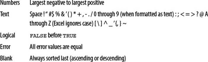
How Excel sorts a table depends on the data. Here’s the order Excel uses in an ascending sort:
Type (in Order of Priority) Order
Performing a More Complex Sort
For more complex sorts on multiple fields, follow these steps:
1. Select a cell inside a table.
2. Select Data, Sort. Excel displays the Sort dialog box, shown in Figure 13.3.
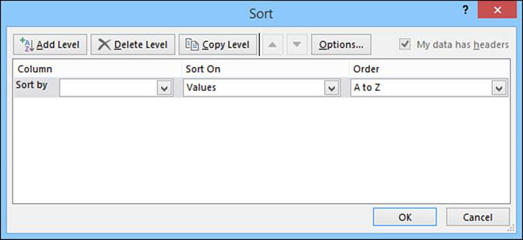
Figure 13.3 Use the Sort dialog box to sort a table on one or more fields.
3. Use the Sort By list to select the field you want to use for the overall order for the sort.
4. Use the Order list to select either an ascending or descending sort.
5. (Optional) If you want to sort the data on more than one field, click Add Level, use the Then By list to click the field, and then select a sort order. Repeat for any other fields you want to include in the sort.
Note
You can specify up to 64 sorting levels.
Caution
Be careful when you sort table records that contain formulas. If the formulas use relative addresses that refer to cells outside their own record, the new sort order might change the references and produce erroneous results. If your table formulas must refer to cells outside the table, be sure to use absolute addresses.
6. (Optional) Click Options to specify one or more of the following sort controls:
• Case Sensitive—Select this check box to have Excel differentiate between uppercase and lowercase during sorting. In an ascending sort, for example, lowercase letters are sorted before uppercase letters.
• Orientation—Excel normally sorts table rows (the Sort Top to Bottom option). To sort table columns, select Sort Left to Right.
7. Click OK. Excel sorts the range.
Sorting a Table in Natural Order
It’s often convenient to see the order in which records were entered into a table, or the natural order of the data. Normally, you can restore a table to its natural order by choosing Undo Sort in the Quick Access Toolbar immediately after a sort.
Unfortunately, after several sort operations, it’s no longer possible to restore the natural order. The solution in this case is to create a new field, such as a field called Record, in which you assign consecutive numbers as you enter the data. The first record is 1, the second is 2, and so on. To restore the table to its natural order, you sort on the Record field.
Caution
The Record field works only if you add it either before you start inserting new records in the table or before you’ve irrevocably sorted the table. Therefore, when planning any table, you might consider always including a Record field just in case you need it.
Follow these steps to add a new field to a table:
1. Select a cell in the field to the right of where you want the new field inserted.
2. In the Home tab, select Insert, Table Columns to the Left. Excel inserts the column.
3. Rename the column header to the field name you want to use.
Figure 13.4 shows the accounts receivable table with a Record field added and the record numbers inserted.
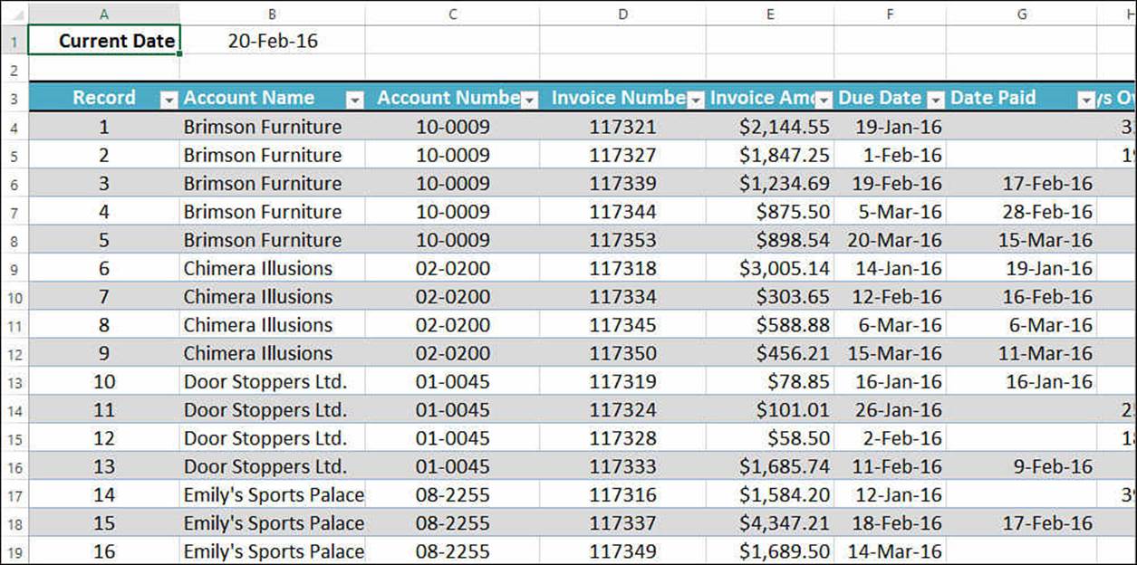
Figure 13.4 The Record field tracks the order in which records are added to a table.
Tip
If you’re not sure how many records are in the table, and if the table isn’t sorted in natural order, you might not know which record number to use next. To avoid guessing or searching through the entire Record field, you can generate the record numbers automatically by using the MAX() function. Click the formula bar and type (but don’t confirm) the following:
=MAX(Column:Column)
Replace Column with the letter of the column that contains the record number (for example, MAX(A:A) for the table in Figure 13.4). Now select the formula and press F9. Excel displays the formula result, which will be the highest record number used so far. Therefore, your next record number will be one more than the calculated value.
Sorting on Part of a Field
Excel performs its sorting chores based on the entire contents of each cell in a field. This method is fine for most sorting tasks, but occasionally you need to sort on only part of a field. For example, your table might have a ContactName field that contains a first name and then a last name. Sorting on this field orders the table by each person’s first name, which is probably not what you want. To sort on the last name, you need to create a new column that extracts the last name from the ContactName field. You can then use this new column for the sort.
Excel’s text functions make it easy to extract substrings from a cell. In this case, assume that each cell in the ContactName field has a first name, followed by a space, followed by a last name. Your task is to extract everything after the space, and the following formula does the job (assuming that the name is in cell D4):
=RIGHT(D4, LEN(D4) - FIND(" ", D4))
![]() For an explanation of how this formula works, see “Extracting a First Name or Last Name,” p. 156.
For an explanation of how this formula works, see “Extracting a First Name or Last Name,” p. 156.
Figure 13.5 shows this formula in action. Column D contains the names, and column A contains the formula to extract the last name. I sorted on column A to order the table by last name.
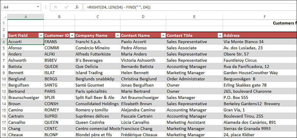
Figure 13.5 To sort on part of a field, use Excel’s text functions to extract the string you need for the sort.
Tip
If you’d rather not have the extra sort field (column A in Figure 13.5) cluttering the table, you can hide it by selecting a cell in the field and choosing Home, Format, Hide & Unhide, Hide Columns. Fortunately, you don’t have to unhide the field to sort on it because Excel still includes the field in the Sort By table.
Sorting Without Articles
Tables that contain field values starting with articles (A, An, and The) can throw off your sorting. To fix this problem, you can borrow the technique from the preceding section and sort on a new field in which the leading articles have been removed. As before, you want to extract everything after the first space, but you can’t just use the same formula because not all the titles have a leading article. You need to test for a leading article by using the following OR() function:
OR(LEFT(A2,2) = "A ", LEFT(A2,3) = "An ", LEFT(A2,4) = "The ")
Here, I’m assuming that the text being tested is in cell A2. If the left two characters are A followed by a space, or the left three characters are An followed by a space, or the left four characters are The followed by a space, this function returns TRUE. (That is, you’re dealing with a title that has a leading article.)
Now you need to package this OR() function inside an IF() test. If the OR() function returns TRUE, the command should extract everything after the first space; otherwise, it should just return the entire title. Here it is:
=IF( OR(LEFT(A2,2) = "A ", LEFT(A2,3) = "An ", LEFT(A2,4) = "The "), RIGHT(A2, LEN(A2) - FIND(" ", A2, 1)), A2)
Figure 13.6 shows this formula in action.
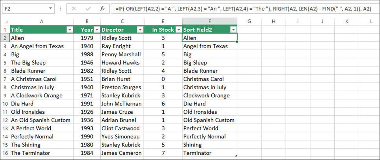
Figure 13.6 A formula that removes leading articles for proper sorting.
Filtering Table Data
One of the biggest problems with large tables is that it’s often hard to find and extract the data you need. Sorting can help, but in the end, you’re still working with the entire table. What you need is a way to define the data that you want to work with and then have Excel display only those records onscreen. This is called filtering your data, and Excel offers several techniques that get the job done.
Using Filter Lists to Filter a Table
Excel’s Filter feature makes filtering out subsets of your data as easy as selecting an option from a drop-down list. In fact, that’s literally what happens. When you convert a range to a table, Excel automatically turns on the Filter feature, which is why you see drop-down arrows in the cells containing the table’s column labels. (You can toggle Filter off and on by choosing Data, Filter.) Clicking one of these arrows displays a table of all the unique entries in the column. Figure 13.7 shows the drop-down table for the Account Name field in the accounts receivable table.
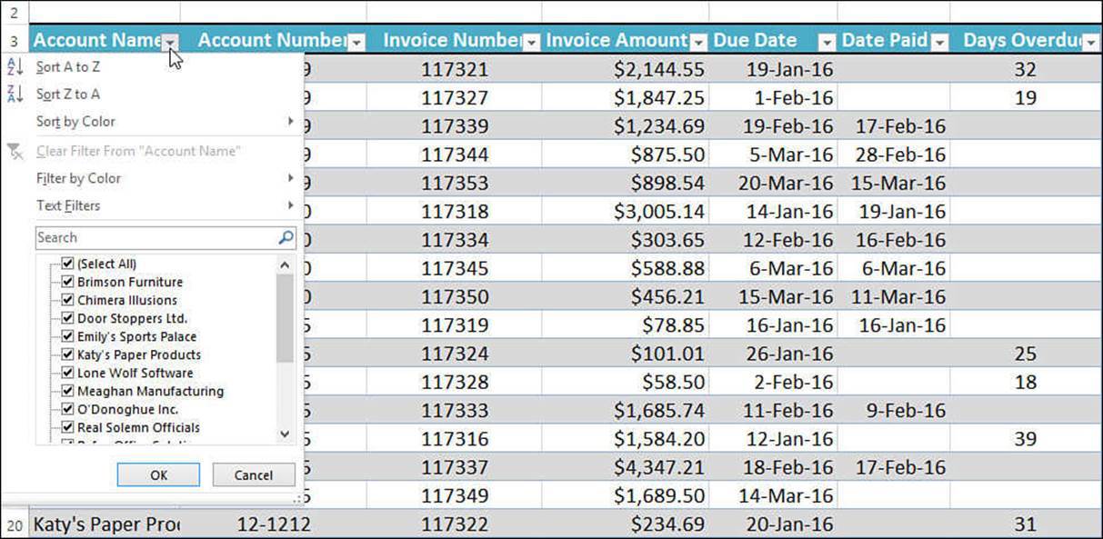
Figure 13.7 For each table field, Filter adds drop-down lists that contain only the unique entries in the column.
There are two basic techniques you can use in a Filter list:
![]() Deselect an item’s check box to hide that item in the table.
Deselect an item’s check box to hide that item in the table.
![]() Click to deselect the Select All item, which deselects all the check boxes, and then click to select the check box for each item you want to see in the table.
Click to deselect the Select All item, which deselects all the check boxes, and then click to select the check box for each item you want to see in the table.
For example, Figure 13.8 shows the resulting records when I deselect all the check boxes and then select only the check boxes for Brimson Furniture and Katy’s Paper Products. The other records are hidden and can be retrieved whenever needed. To continue filtering the data, you can select an item from one of the other tables. For example, you could select a month from the Due Date list to see only the invoices due within that month.
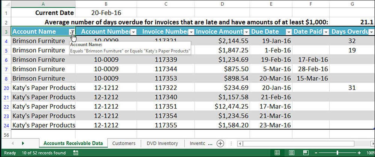
Figure 13.8 Clicking an item in a Filter drop-down list displays only records that include the item in the field.
Caution
Because Excel hides the rows that don’t meet the criteria, you shouldn’t place any important data either to the left or to the right of the table.
Here are three things to notice about a filtered table:
![]() Excel reminds you that the table is filtered on a particular column by adding a funnel icon to the column’s drop-down list button.
Excel reminds you that the table is filtered on a particular column by adding a funnel icon to the column’s drop-down list button.
![]() You can see the exact filter by hovering the mouse over the filtered column’s drop-down button. As you can see in Figure 13.8, Excel displays a banner that tells you the filter criteria.
You can see the exact filter by hovering the mouse over the filtered column’s drop-down button. As you can see in Figure 13.8, Excel displays a banner that tells you the filter criteria.
![]() Excel also displays a message in the status bar telling you the number of records it filtered (again, refer to Figure 13.8).
Excel also displays a message in the status bar telling you the number of records it filtered (again, refer to Figure 13.8).
Working with Quick Filters
The items you see in each drop-down table are called the filter criteria. Besides selecting specific criteria (such as an account name), Excel also offers a set of quick filters that enable you to apply specific criteria. The quick filters you see depend on the data type of the field, but in each case you access them by pulling down a field’s Filter drop-down list:
![]() Text Filters—This command appears when you’re working with a text field. It displays a submenu of filters that includes Equals, Does Not Equal, Begins With, Ends With, Contains, and Does Not Contain.
Text Filters—This command appears when you’re working with a text field. It displays a submenu of filters that includes Equals, Does Not Equal, Begins With, Ends With, Contains, and Does Not Contain.
![]() Number Filters—This command appears when you’re working with a numeric field. It displays a submenu of filters that includes Equals, Does Not Equal, Greater Than, Less Than, Between, Top 10, Above Average, and Below Average.
Number Filters—This command appears when you’re working with a numeric field. It displays a submenu of filters that includes Equals, Does Not Equal, Greater Than, Less Than, Between, Top 10, Above Average, and Below Average.
![]() Date Filters—This command appears when you’re working with a date field. It displays a submenu of filters that includes Equals, Before, After, Between, Tomorrow, Today, Next Week, This Month, Last Year, and many others. Figure 13.9 shows the Date Filters menu that appears for the accounts receivable table.
Date Filters—This command appears when you’re working with a date field. It displays a submenu of filters that includes Equals, Before, After, Between, Tomorrow, Today, Next Week, This Month, Last Year, and many others. Figure 13.9 shows the Date Filters menu that appears for the accounts receivable table.
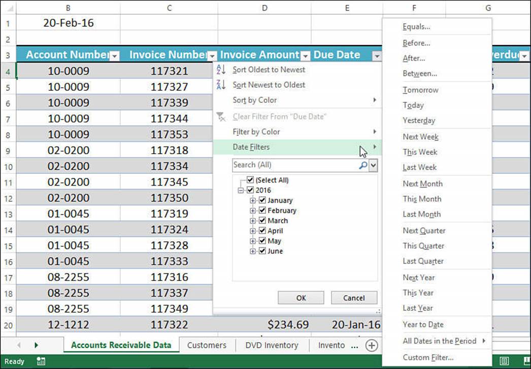
Figure 13.9 For a date field, the Date Filters command offers a wide range of quick filters that you can apply.
Whichever quick filter you select (or if you click the Custom Filter command that appears at the bottom of each quick filter menu), Excel displays the Custom AutoFilter dialog box, an example of which is shown in Figure 13.10.
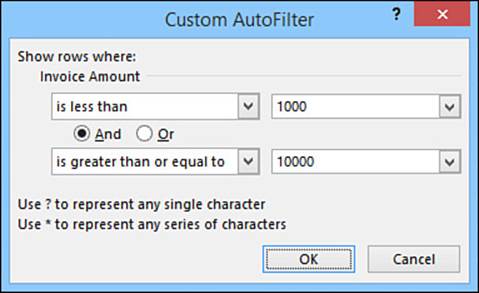
Figure 13.10 Use the Custom AutoFilter dialog box to specify your quick filter criteria or enter custom criteria.
You use the two drop-down lists across the top to set up the first part of your criterion. The drop-down on the left contains a list of Excel’s comparison operators (such as Equals and Is Greater Than). The combo box on the right enables you to select a unique item from the field or enter your own value. For example, if you want to display invoices with an amount less than $1,000, click the Is Less Than operator and enter 1000 in the text box.
For text fields, you also can use wildcard characters to substitute for one or more characters. Use the question mark (?) wildcard to substitute for a single character. For example, if you enter sm?th, Excel finds both Smith and Smyth. To substitute for groups of characters, use the asterisk (*). For example, if you enter *carolina, Excel finds all the entries that end with “carolina.”
Tip
To include a wildcard as part of the criteria, precede the character with a tilde (~). For example, to find OVERDUE?, enter OVERDUE~?.
You can create compound criteria by clicking the And or Or button and then entering another criterion in the bottom two drop-down lists. Use And when you want to display records that meet both criteria; use Or when you want to display records that meet at least one of the two criteria.
For example, to display invoices with an amount less than $1,000 and greater than or equal to $10,000, you fill in the dialog box as shown in Figure 13.10.
Showing Filtered Records
When you need to redisplay records that have been filtered via Filter, use any of the following techniques:
![]() To display the entire table and remove the Filter feature’s drop-down arrows, deselect the Data, Filter command.
To display the entire table and remove the Filter feature’s drop-down arrows, deselect the Data, Filter command.
![]() To display the entire table without removing the Filter drop-down arrows, select Data, Clear.
To display the entire table without removing the Filter drop-down arrows, select Data, Clear.
![]() To remove the filter on a single field, display that field’s Filter drop-down list and select the Clear Filter from Field command, where Field is the name of the field.
To remove the filter on a single field, display that field’s Filter drop-down list and select the Clear Filter from Field command, where Field is the name of the field.
Using Complex Criteria to Filter a Table
The Filter feature should take care of most of your filtering needs, but it’s not designed for heavy-duty work. For example, Filter can’t handle the following accounts receivable criteria:
![]() Invoice amounts greater than $100, less than $1,000, or greater than $10,000
Invoice amounts greater than $100, less than $1,000, or greater than $10,000
![]() Account numbers that begin with 01, 05, or 12
Account numbers that begin with 01, 05, or 12
![]() Days overdue greater than the value in cell J1
Days overdue greater than the value in cell J1
To work with these more sophisticated requests, you need to use complex criteria.
Setting Up a Criteria Range
Before you can work with complex criteria, you must set up a criteria range. A criteria range has some or all of the table field names in the top row, with at least one blank row directly underneath. You enter your criteria in the blank row below the appropriate field name, and Excel searches the table for records with field values that satisfy the criteria. This setup gives you two major advantages over Filter:
![]() By using either multiple rows or multiple columns for a single field, you can create compound criteria with as many terms as you like.
By using either multiple rows or multiple columns for a single field, you can create compound criteria with as many terms as you like.
![]() Because you’re entering your criteria in cells, you can use formulas to create computed criteria.
Because you’re entering your criteria in cells, you can use formulas to create computed criteria.
You can place the criteria range anywhere on the worksheet outside the table range. The most common position, however, is a couple of rows above the table range. Figure 13.11 shows the accounts receivable table with a criteria range (A2:G3). As you can see, the criteria are entered in the cell below the field name. In this case, the displayed criteria will find all Brimson Furniture invoices that are greater than or equal to $1,000 and that are overdue (that is, invoices that have a value greater than 0 in the Days Overdue field).
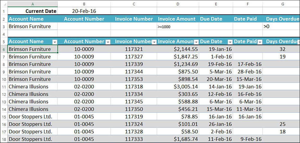
Figure 13.11 Set up a separate criteria range (A2:G3, in this case) to enter complex criteria.
Filtering a Table with a Criteria Range
After you’ve set up your criteria range, you can use it to filter the table. The following steps take you through the basic procedure:
1. Copy the table field names that you want to use for the criteria and paste them into the first row of the criteria range. If you’ll be using different fields for different criteria, consider copying all your field names into the first row of the criteria range.
Tip
The only problem with copying the field names to the criteria range is that if you change a field name, you must change it in two places (that is, in the table and in the criteria). So, instead of just copying the names, you can make the field names in the criteria range dynamic by using a formula to set each criteria field name equal to its corresponding table field name. For example, you could enter =B5 in cell B2 of Figure 13.11.
2. Below each field name in the criteria range, enter the criteria you want to use.
3. Select a cell in the table and then select Data, Advanced. Excel displays the Advanced Filter dialog box, shown in Figure 13.12.
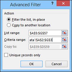
Figure 13.12 Use the Advanced Filter dialog box to select your table and criteria ranges.
4. Ensure that the List Range text box contains the table range (which it should if you selected a cell in the table beforehand). If it doesn’t, select the text box and select the table (including the field names).
5. In the Criteria Range text box, select the criteria range (again, including the field names you copied).
6. To avoid including duplicate records in the filter, select the Unique Records Only check box.
7. Click OK. Excel filters the table to show only those records that match your criteria (see Figure 13.13).
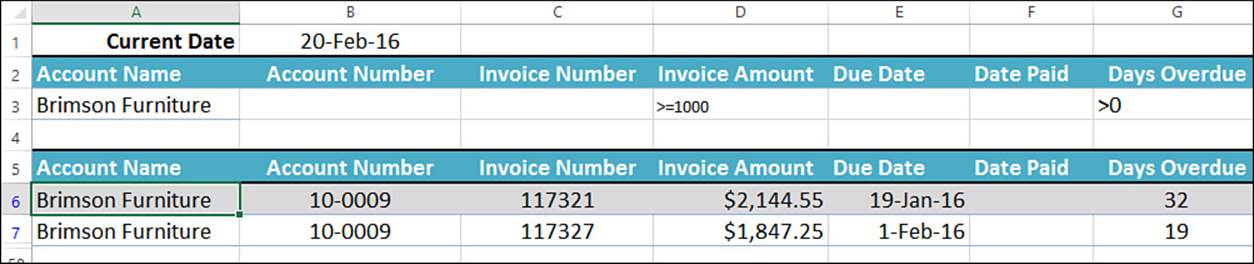
Figure 13.13 The accounts receivable table filtered using the complex criteria specified in the criteria range.
Entering Compound Criteria
To enter compound criteria in a criteria range, use the following guidelines:
![]() To find records that match all the criteria, enter the criteria on a single row.
To find records that match all the criteria, enter the criteria on a single row.
![]() To find records that match one or more of the criteria, enter the criteria on separate rows.
To find records that match one or more of the criteria, enter the criteria on separate rows.
Finding records that match all the criteria is equivalent to activating the And button in the Custom AutoFilter dialog box. The sample criteria shown in Figure 13.11 match records with the account name Brimson Furniture and an invoice amount greater than $1,000 and a positive number in the Days Overdue field. To narrow the displayed records, you can enter criteria for as many fields as you like.
Tip
You can use the same field name more than once in compound criteria. To do this, you include the appropriate field multiple times in the criteria range and enter the appropriate criteria below each label.
Finding records that match at least one of several criteria is equivalent to activating the Or button in the Custom AutoFilter dialog box. In this case, you need to enter each criterion on a separate row. For example, to display all invoices with amounts greater than or equal to $10,000 or that are more than 30 days overdue, you would set up your criteria as shown in Figure 13.14.
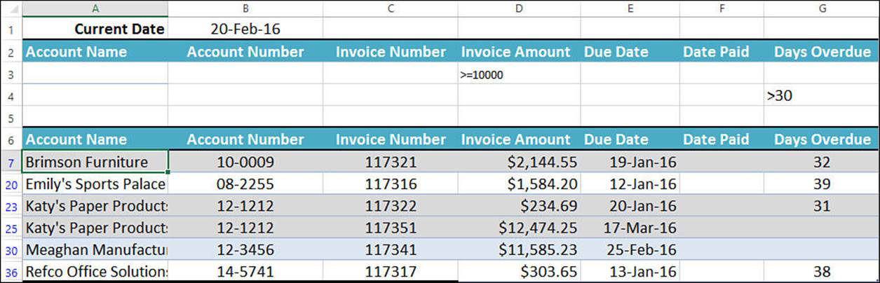
Figure 13.14 To display records that match one or more of the criteria, enter the criteria in separate rows.
Caution
Don’t include any blank rows in your criteria range because blank rows throw off Excel when it tries to match the criteria.
Entering Computed Criteria
The fields in your criteria range aren’t restricted to the table fields. You can create computed criteria that use a calculation to match records in the table. The calculation can refer to one or more table fields, or even to cells outside the table, and must return either TRUE or FALSE. Excel selects records that return TRUE.
To use computed criteria, add a column to the criteria range and enter the formula in the new field. Make sure that the name you give the criteria field is different from any field name in the table. When referencing the table cells in the formula, use the first data row of the table. For example, to select all records in which Date Paid is equal to Due Date in the accounts receivable table, enter the following formula:
=F6=E6
Note the use of relative addressing. If you want to reference cells outside the table, use absolute addressing.
Tip
Use Excel’s AND, OR, and NOT functions to create compound computed criteria. For example, to select all records in which the Days Overdue value is less than 90 and greater than 31, type this:
=AND(G6<90, G6>31)
Figure 13.15 shows a more complex example. The goal is to select all records whose invoices were paid after the due date. The new criterion—named Late Payers—contains the following formula:
=IF(ISBLANK(F6), FALSE(), F6 > E6)
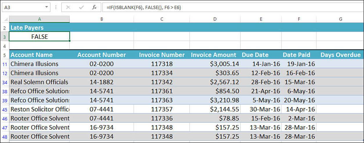
Figure 13.15 Use a separate criteria range column for calculated criteria.
If the Date Paid field (column F) is blank, the invoice hasn’t been paid, so the formula returns FALSE. Otherwise, the logical expression F6 > E6 is evaluated. If the Date Paid field (column F) is greater than the Due Date field (column E), the expression returns TRUE, and Excel selects the record. In Figure 13.15, the Late Payers cell (A3) displays FALSE because the formula evaluates to FALSE for the first row in the table.
Copying Filtered Data to a Different Range
If you want to work with the filtered data separately, you can copy it (or extract it) to a new location. Follow these steps:
1. Set up the criteria you want to use to filter the table.
2. If you want to copy only certain columns from the table, copy the appropriate field names to the range you’ll be using for the copy.
3. Select Data, Advanced to display the Advanced Filter dialog box.
4. Select the Copy to Another Location option.
5. Enter your table and criteria ranges, if necessary.
6. Use the Copy To box to enter a reference for the copy location, using the following guidelines. (Note that, in each case, you must select the cell or range in the same worksheet that contains the table.)
• To copy the entire filtered table, enter a single cell.
• To copy only a specific number of rows, enter a range that contains the number of rows you want. If you have more data than fits in the range, Excel asks whether you want to paste the remaining data.
• To copy only certain columns, select the column labels you copied in step 2.
Caution
If you select a single cell in which to paste the entire filtered table, make sure you won’t be overwriting any data. Otherwise, Excel copies over the data without warning.
7. Click OK. Excel filters the table and copies the selected records to the location you specified.
Figure 13.16 shows the results of an extract in the accounts receivable table.
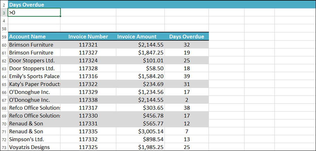
Figure 13.16 This filter operation selects those records in which the Days Overdue field is greater than 0 and then copies the results to a range below the table.
Referencing Tables in Formulas
In legacy versions of Excel, when you needed to reference part of a table in a formula, you usually just used a cell or range reference that pointed to the area within the table that you wanted to use in your calculation. That worked, but it suffered from the same problem caused by using cell and range references in regular worksheet formulas: The references often make the formulas difficult to read and understand. The solution with a regular worksheet formula is to replace cell and range references with defined names, but Excel offered no easy way to use defined names with tables.
That all changed beginning with Excel 2007 because the program now supports structured referencing of tables. This means that Excel offers a set of defined names—or specifiers, as Microsoft calls them—for various table elements (such as the data, the headers, and the entire table), as well as the automatic creation of names for the table fields. You can include these names in your table formulas to make your calculations much easier to read and maintain.
Using Table Specifiers
First, let’s look at the predefined specifiers that Excel offers for tables. Table 13.1 lists the names you can use.
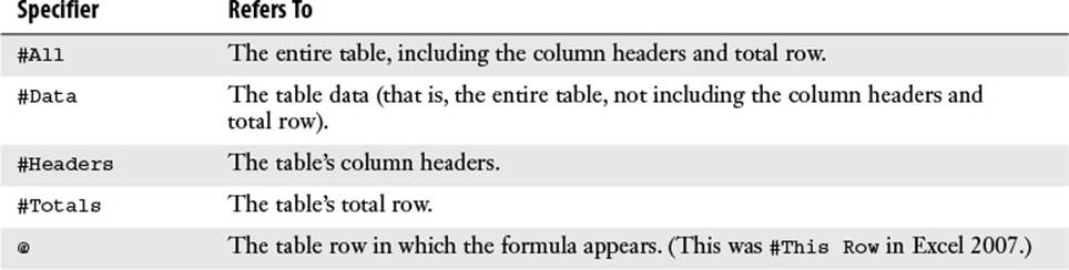
Table 13.1 Excel’s Predefined Table Specifiers
Most table references start with the table name (as given by the Design, Table Name property). In the simplest case, you can just use the table name by itself. For example, the following formula counts the numeric values in a table named Table1:
=COUNT(Table1)
If you want to reference a specific part of the table, you must enclose that reference in square brackets after the table name. For example, the following formula calculates the maximum data value in a table named Sales:
=MAX(Sales[#Data])
Tip
You can also reference tables in other workbooks by using the following syntax:
'Workbook'!Table
Here, replace Workbook with the workbook filename and replace Table with the table name.
Note
Using just the table name by itself is equivalent to using the #Data specifier. So, for example, the following two formulas produce the same result:
=MAX(Sales[#Data])
=MAX(Sales)
Excel also generates column specifiers based on the text in the column headers. Each column specifier references the data in the column, so it doesn’t include the column’s header or total. For example, suppose you have a table named Inventory, and you want to calculate the sum of the values in the field named Qty On Hand. The following formula does the trick:
=SUM(Inventory[Qty On Hand])
If you want to refer to a single value in a table field, you need to specify the row you want to work with. Here’s the general syntax for this:
Table[[Row],[Field]]
Here, replace Table with the table name, Row with a row specifier, and Field with a field specifier. For the row specifier, you have only two choices: the current row and the totals row. The current row is the row in which the formula resides, and in Excel 2010 and later you use the @specifier to designate the current row (in Excel 2007, this specifier was #This Row). In this case, however, you use @ followed by the name of the field in square brackets, like so:
@[Standard Cost]
For example, in a table named Inventory with a field named Standard Cost, the following formula multiplies the Standard Cost value in the current row by 1.25:
=Inventory[@[Standard Cost]] * 1.25
Note
If your formula needs to reference a cell in a row other than the current row or the totals row, you need to use a regular cell reference such as A3 or D6.
For a cell in the totals row, use the #Totals specifier, as in this example:
=Inventory[[#Totals],[Qty On Hand]] - Inventory[[#Totals],[Qty On Hold]]
Finally, you can also create ranges by using structured table referencing. As with regular cell references, you create a range by inserting a colon between two specifiers. For example, the following reference includes all the data cells in the Inventory table’s Qty On Hold and Qty On Hand fields:
Inventory[[Qty On Hold]:[Qty On Hand]]
Entering Table Formulas
When you build a formula using structured referencing, Excel offers several tools that make it easy and accurate. First, note that table names are part of Excel’s Formula AutoComplete feature. This means that after you type the first few letters of the table name, you’ll see the formula name in the AutoComplete list, so you can then select the name and press Tab to add it to your formula. When you then type the opening square bracket ([), Excel displays a list of the table’s available specifiers, as shown in Figure 13.17. The first few items are the field names, and the bottom five are the built-in specifiers. Select the specifier and press Tab to add it to your formula. Each time you type an opening square bracket, Excel displays the specifier list.
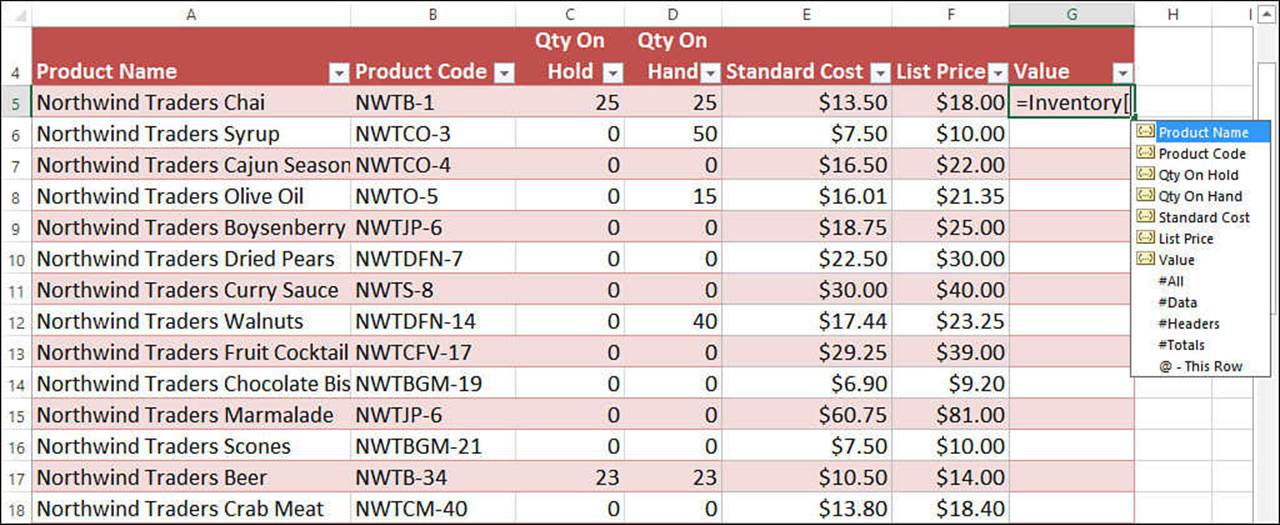
Figure 13.17 Type a table name and the opening square bracket ([), and Excel displays a list of the table’s specifiers.
One of my favorite Excel features is its support for automatic calculated columns. To demonstrate how this works, Figure 13.18 shows a full formula that I’ve typed into a table cell but haven’t yet completed (by, say, pressing Enter). When I press Enter, Excel automatically fills the same formula down into the rest of the table’s rows, as you can see in Figure 13.19. Excel also displays an AutoCorrect Options button, which enables you to reverse the calculated column, if desired.
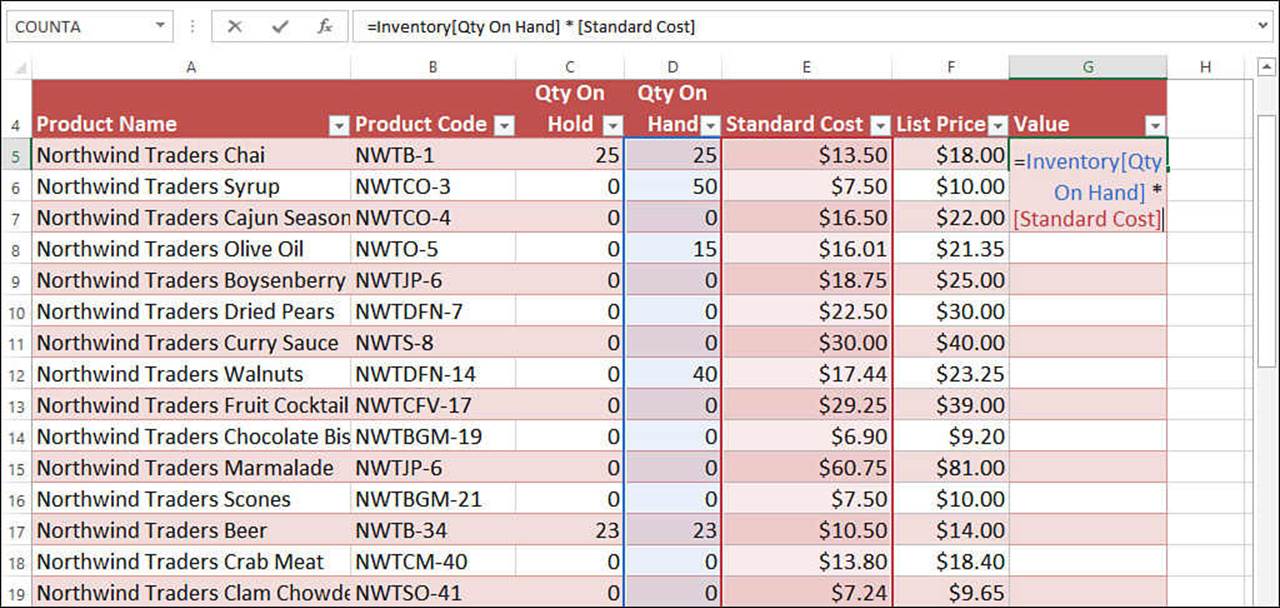
Figure 13.18 A new table formula, ready to be confirmed.
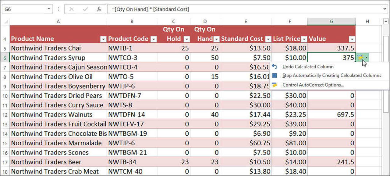
Figure 13.19 When you confirm a new table formula, Excel automatically fills the formula down into the rest of the table.
Note
In Figure 13.19, notice also that Excel simplified the table formula by removing the table names, which it considers redundant.
Excel’s Table Functions
To take your table analysis to a higher level, you can use Excel’s table functions, which give you the following advantages:
![]() You can enter the functions into any cell in the worksheet.
You can enter the functions into any cell in the worksheet.
![]() You can specify the range the function uses to perform its calculations.
You can specify the range the function uses to perform its calculations.
![]() You can enter criteria or reference a criteria range to perform calculations on subsets of the table.
You can enter criteria or reference a criteria range to perform calculations on subsets of the table.
About Table Functions
To illustrate the table functions, consider an example: If you want to calculate the sum of a table field, you can enter SUM(range), and Excel produces the result. If you want to sum only a subset of the field, you must specify as arguments the particular cells to use. For tables containing hundreds of records, however, this process is impractical.
The solution is to use DSUM(), which is the table equivalent of the SUM() function. The DSUM() function takes three arguments: a table range, field name, and criteria range. DSUM() looks at the specified field in the table and sums only records that match the criteria in the criteria range.
The table functions come in two varieties: those that don’t require a criteria range and those that do.
Table Functions That Don’t Require a Criteria Range
Excel has three table functions that enable you to specify the criteria as an argument rather than a range: COUNTIF(), SUMIF(), and AVERAGEIF().
Using COUNTIF()
The COUNTIF() function counts the number of cells in a range that meet a single criteria:
COUNTIF(range, criteria)
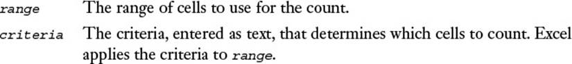
For example, Figure 13.20 shows a COUNTIF() function that calculates the total number of products that have no stock (that is, where the Qty On Hand field equals zero).
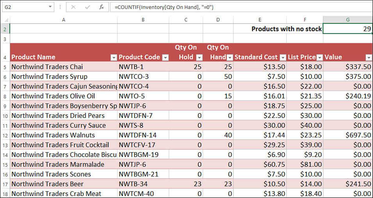
Figure 13.20 Use COUNTIF() to count the cells that meet a criteria.
Using SUMIF()
The SUMIF() function is similar to COUNTIF(), except that it sums the range cells that meet its criteria:
SUMIF(range, criteria[, sum_range])
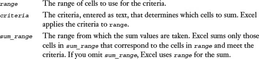
Figure 13.21 shows a Parts table. The SUMIF() function in cell F16 sums the Total Cost field for the parts where the Division field is equal to 3.
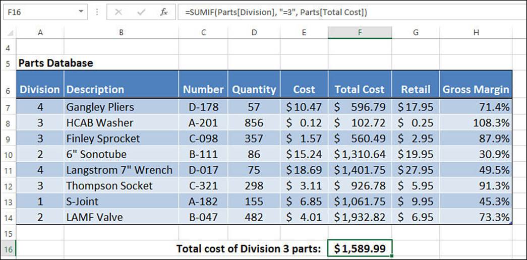
Figure 13.21 Use SUMIF() to sum cells that meet a criteria.
Using AVERAGEIF()
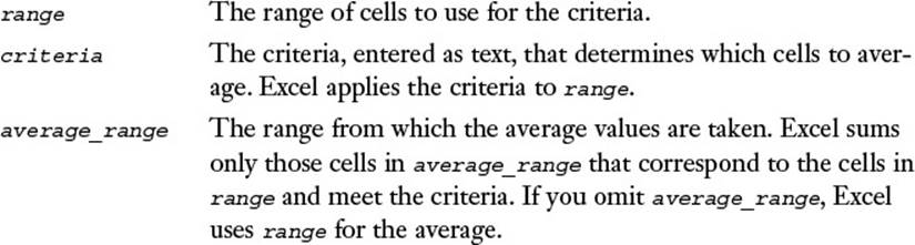
The AVERAGEIF() function calculates the average of a range of cells that meet its criteria:
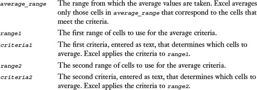
AVERAGEIF(range, criteria[, average_range])
In Figure 13.22, the AVERAGEIF() function in cell F17 averages the Gross Margin field for the parts where the Cost field is less than 10.
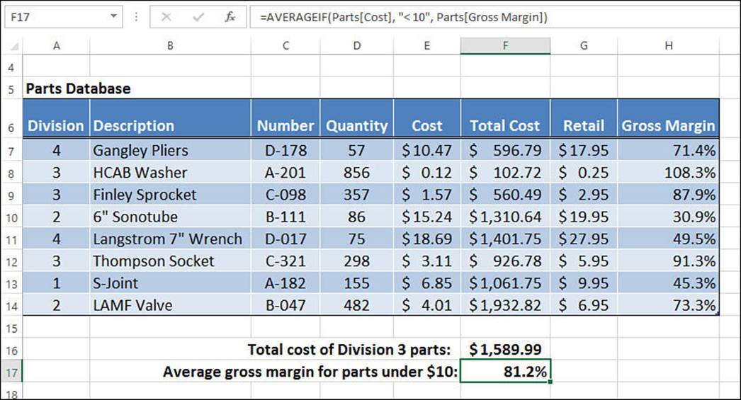
Figure 13.22 Use AVERAGEIF() to sum cells that meet a criteria.
Using AGGREGATE()
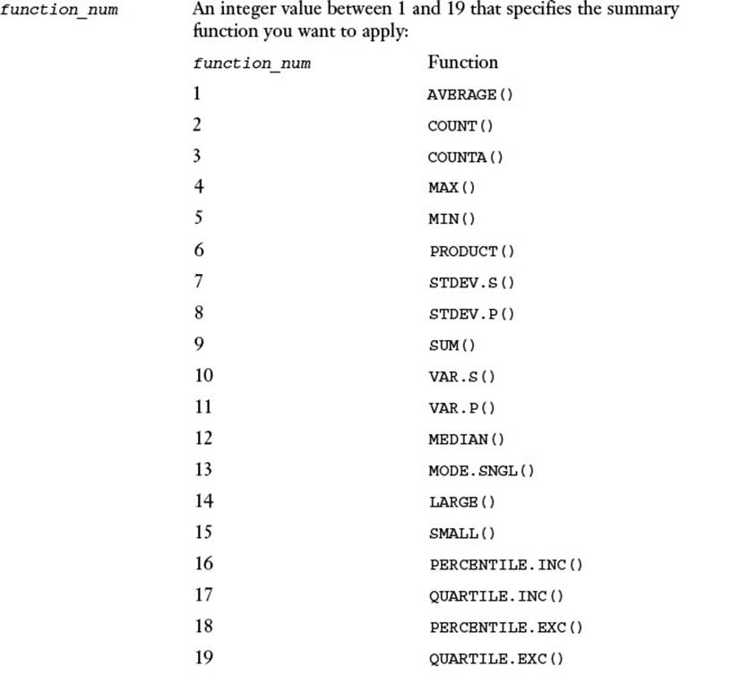
The AGGREGATE() function is an all-purpose tool that can return a result for one of 19 summary functions—including AVERAGE(), SUM(), COUNT(), and the functions associated with variance and standard deviation—applied to the data in a numeric range. Here’s the syntax:
AGGREGATE(function_num, options, ref1[, ref2,...])
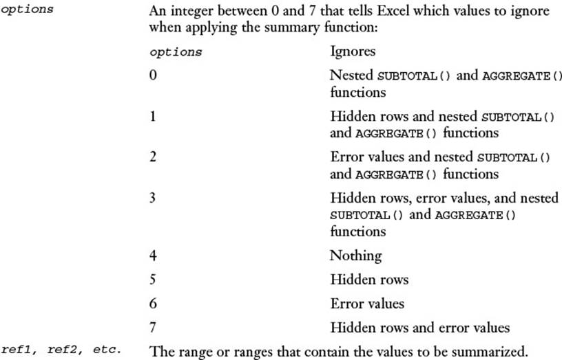
For example, the following formula calculates the largest value in the range A2:A100 while ignoring hidden rows and error values:
=AGGREGATE(14, 7, A2:A100)
Table Functions That Accept Multiple Criteria
In legacy versions of Excel, if you wanted to sum table values that satisfy two or more criteria, it was possible, but it usually required jumping through some serious formula hoops. For example, you could nest multiple IF() functions inside a SUM() function entered as an array formula. In other words, it was doable, but it wasn’t for the faint of heart.
Beginning with Excel 2007, this was fixed, and Excel now offers three functions that enable you to specify multiple criteria: COUNTIFS(), SUMIFS(), and AVERAGEIFS(). Note that none of these functions requires a separate criteria range.
Using COUNTIFS()
The COUNTIFS() function counts the number of cells in one or more ranges that meet one or more criteria:
COUNTIFS(range1, criteria1[, range2, criteria2, ...])
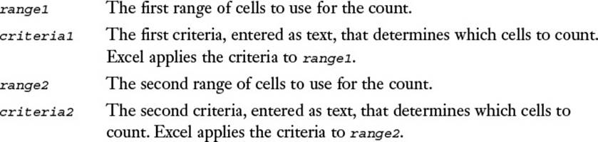
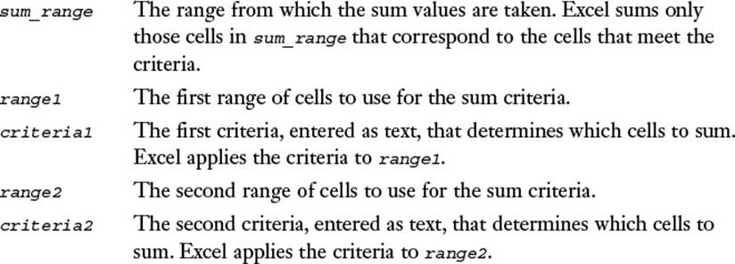
You can enter up to 127 range/criteria pairs. For example, Figure 13.23 shows a COUNTIFS() function in cell H1 that returns the number of customers where the Country field equals USA and the Region field equals OR. (This is short for Oregon; don’t confuse it with Excel’s OR()function!)
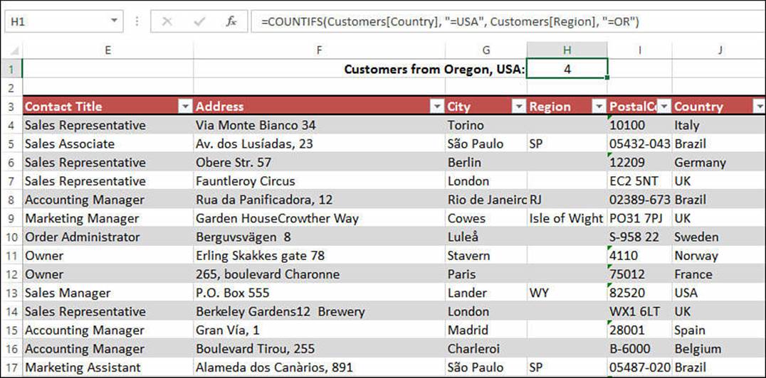
Figure 13.23 Use COUNTIFS() to count the cells that meet one or more criteria.
Using SUMIFS()
The SUMIFS() function sums cells in one or more ranges that meet one or more criteria:
SUMIFS(sum_range, range1, criteria1[, range2, criteria2, ...])
You can enter up to 127 range/criteria pairs. Figure 13.24 shows the Inventory table. The SUMIFS() function in cell G1 sums the Qty On Hand field for the products where the Product Name field includes Soup and the Qty On Hold field equals zero.
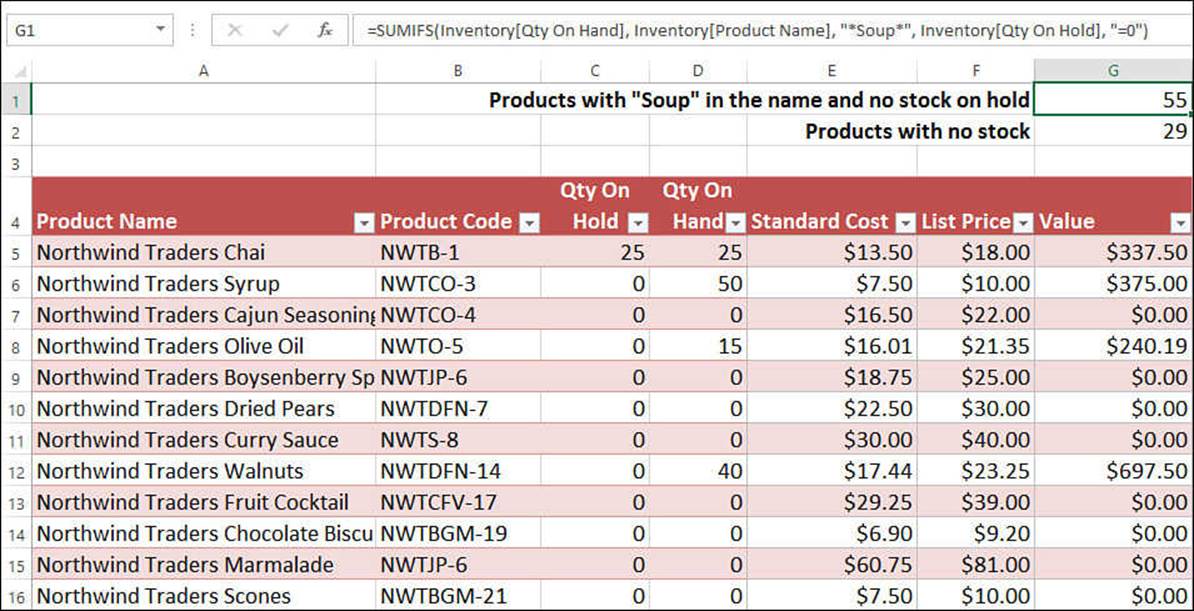
Figure 13.24 Use SUMIFS() to sum the cells that meet one or more criteria.
Using AVERAGEIFS()
The AVERAGEIFS() function averages cells in one or more ranges that meet one or more criteria:
AVERAGEIFS(average_range, range1, criteria1[, range2, criteria2, ...])
You can enter up to 127 range/criteria pairs. Figure 13.25 shows the accounts receivable table. The AVERAGEIFS() function in cell G2 averages the Days Overdue field for the invoices where the Days Overdue is greater than 0 and where the Invoice Amount field is greater than or equal to 1000.
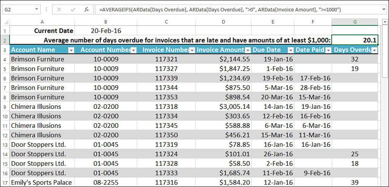
Figure 13.25 Use AVERAGEIFS() to average the cells that meet one or more criteria.
Table Functions That Require a Criteria Range
The remaining table functions require a criteria range. These functions take a little longer to set up, but the advantage is that you can enter compound and computed criteria.
All of these functions have the following format:
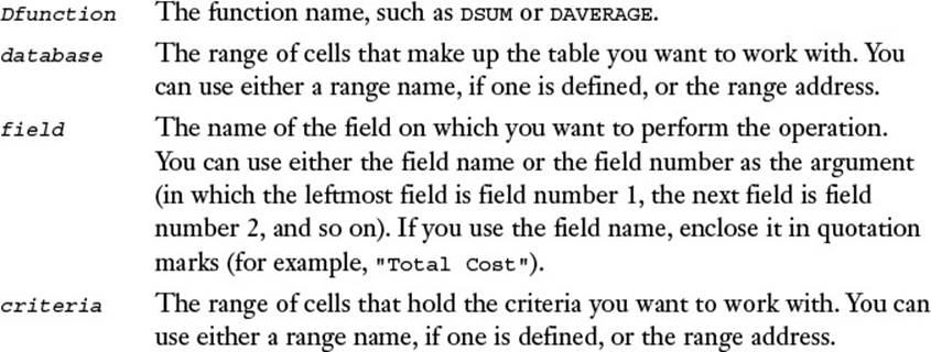
Dfunction(database, field, criteria)
Tip
To perform an operation on every record in a table, leave all the criteria fields blank. This causes Excel to select every record in the table.
Table 13.2 summarizes the table functions.
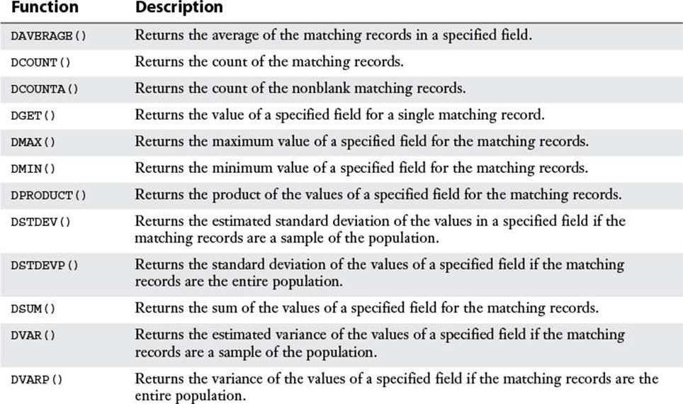
Table 13.2 Excel’s Table Functions
![]() To learn about statistical operations such as standard deviation and variance, see Chapter 12, “Working with Statistical Functions,” p. 257.
To learn about statistical operations such as standard deviation and variance, see Chapter 12, “Working with Statistical Functions,” p. 257.
You enter table functions the same way you enter any other Excel function. You type an equal sign (=) and then enter the function—either by itself or combined with other Excel operators in a formula. The following examples show valid table functions:
=DSUM(A6:H14, "Total Cost", A1:H3)
=DSUM(Table, "Total Cost", Criteria)
=DSUM(AR_Table, 3, Criteria)
=DSUM(1993_Sales, "Sales", A1:H13)
The next two sections provide examples of the DAVERAGE() and DGET() table functions.
Using DAVERAGE()
The DAVERAGE() function calculates the average field value in the database records that match the criteria. In the Parts database, for example, suppose that you want to calculate the average gross margin for all parts assigned to Division 2. You set up a criteria range for the Division field and enter 2, as shown in Figure 13.26. You then enter the following DAVERAGE() function (see cell H3):
=DAVERAGE(Parts[#All], "Gross Margin", A2:A3)
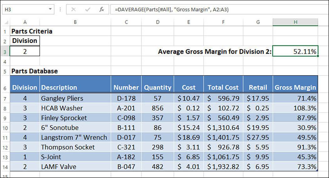
Figure 13.26 Use DAVERAGE() to calculate the field average in the matching records.
Using DGET()
The DGET() function extracts the value of a single field in the database records that match the criteria. If there are no matching records, DGET() returns #VALUE!. If there’s more than one matching record, DGET() returns #NUM!.
DGET() typically is used to query the table for a specific piece of information. For example, in the Parts table, you might want to know the cost of the Finley Sprocket. To extract this information, you would first set up a criteria range with the Description field and enter Finley Sprocket. You would then extract the information with the following formula (assuming that the table and criteria ranges are named Parts and Criteria, respectively):
=DGET(Parts[#All], "Cost", Criteria)
A more interesting application of this function would be to extract the name of a part that satisfies a certain condition. For example, you might want to know the name of the part that has the highest gross margin. Creating this model requires two steps:
1. Set up the criteria to match the highest value in the Gross Margin field.
2. Add a DGET() function to extract the description of the matching record.
Figure 13.27 shows how this is done. For the criteria, a new field called Highest Margin is created. As the text box shows, this field uses the following computed criteria:
=H7 = MAX(Parts2[Gross Margin])
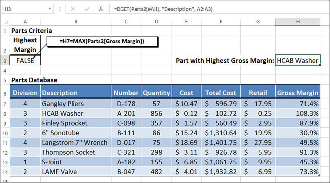
Figure 13.27 A DGET() function that extracts the name of the part with the highest margin.
Excel matches only the record that has the highest gross margin. The DGET() function in cell H3 is straightforward:
=DGET(Parts2[#All], "Description", A2:A3)
This formula returns the description of the part that has the highest gross margin.
Case Study: Applying Statistical Table Functions to a Defects Database
Many table functions are most often used to analyze statistical populations. Figure 13.28 shows a table of defects found among 12 work groups in a manufacturing process. In this example, the table (B3:D15) is named Defects, and two criteria ranges are used—one for each of the group leaders, Johnson (G3:G4 is Criteria1) and Perkins (H3:H4 is Criteria2).
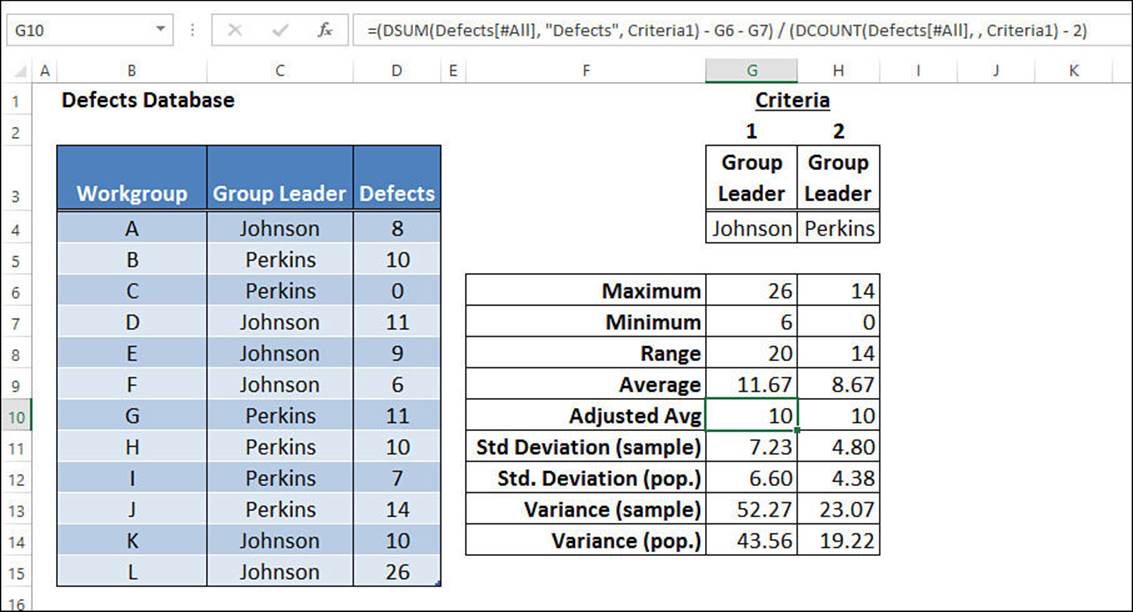
Figure 13.28 Using statistical table functions to analyze a database of defects in a manufacturing process.
The table shows several calculations. First, DMAX() and DMIN() are calculated for each criteria. The range (a statistic that represents the difference between the largest and smallest numbers in the sample; it’s a crude measure of the sample’s variance) is then calculated using the following formula (Johnson’s groups):
=DMAX(Defects[#All], "Defects", Criteria1) - DMIN(Defects[#All],
"Defects", Criteria1)
Of course, instead of using DMAX() and DMIN() explicitly, you can simply refer to the cells containing the DMAX() and DMIN() results.
The next line uses DAVERAGE() to find the average number of defects for each group leader. Notice that the average for Johnson’s groups (11.67) is significantly higher than that for Perkins’s groups (8.67). However, Johnson’s average is skewed higher by one anomalously large number (26), and Perkins’s average is skewed lower by one anomalously small number (0).
To allow for this situation, the Adjusted Avg line uses DSUM(), DCOUNT(), and the DMAX() and DMIN() results to compute a new average without the largest and smallest number for each sample. As you can see, without the anomalies, the two leaders have the same average.
Note
As shown in cell G10 of Figure 13.28, if you don’t include a field argument in the DCOUNT() function, it returns the total number of records in the table.
The rest of the calculations use the DSTDEV(), DSTDEVP(), DVAR(), and DVARP() functions.
From Here
![]() For coverage of the regular SUM() function, see “The SUM() Function,” p. 247.
For coverage of the regular SUM() function, see “The SUM() Function,” p. 247.
![]() For coverage of the regular COUNT() function, see “Counting Items with the COUNT() Function,” p. 261.
For coverage of the regular COUNT() function, see “Counting Items with the COUNT() Function,” p. 261.
![]() For coverage of the regular AVERAGE() function, see “The AVERAGE() Function,” p. 262.
For coverage of the regular AVERAGE() function, see “The AVERAGE() Function,” p. 262.
![]() For more detailed information on statistics such as standard deviation and variance, see Chapter 12, “Working with Statistical Functions,” p. 257.
For more detailed information on statistics such as standard deviation and variance, see Chapter 12, “Working with Statistical Functions,” p. 257.
All materials on the site are licensed Creative Commons Attribution-Sharealike 3.0 Unported CC BY-SA 3.0 & GNU Free Documentation License (GFDL)
If you are the copyright holder of any material contained on our site and intend to remove it, please contact our site administrator for approval.
© 2016-2026 All site design rights belong to S.Y.A.