Excel® 2016 Formulas and Functions (2016)
Part III: Building Business Models
15. Using Excel’s Business Modeling Tools
In This Chapter
Using What-If Analysis
Working with Goal Seek
Working with Scenarios
At times, it’s not enough to simply enter data into a worksheet, build a few formulas, and add a little formatting to make things presentable. In the business world, you’re often called on to divine some inner meaning from the jumble of numbers and formula results that litter your workbooks. In other words, you need to analyze your data to see what nuggets of understanding you can unearth. In Excel, analyzing business data means using the program’s business modeling tools. This chapter looks at a few of those tools and some analytic techniques that have many uses. You’ll find out how to use Excel’s numerous methods for what-if analysis, how to wield Excel’s useful Goal Seek tool, and how to create scenarios.
Using What-If Analysis
What-if analysis is perhaps the most basic method for interrogating your worksheet data. With what-if analysis, you first calculate a formula, D, based on the input from variables A, B, and C. You then say, “What if I change variable A? Or B or C? What happens to the result?”
For example, Figure 15.1 shows a worksheet that calculates the future value of an investment based on five variables: the interest rate, period, annual deposit, initial deposit, and deposit type. Cell C9 shows the result of the FV() function. Now the questions begin:
![]() What if the interest rate is 7%?
What if the interest rate is 7%?
![]() What if you deposit $8,000 per year? Or $12,000?
What if you deposit $8,000 per year? Or $12,000?
![]() What if you reduce the initial deposit?
What if you reduce the initial deposit?
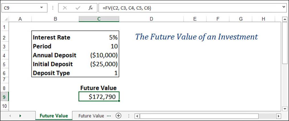
Figure 15.1 The simplest what-if analysis involves changing worksheet variables and watching the result.
Answering these questions is a straightforward matter of changing the appropriate variables and watching the effect on the result.
Note
You can download this chapter’s sample workbook at www.mcfedries.com/books/book.php?title=excel-2016-formulas-and-functions.
Setting Up a One-Input Data Table
The problem with modifying formula variables is that you see only a single result at one time. If you’re interested in studying the effect a range of values has on a formula, you need to set up a data table. In the investment analysis worksheet, for example, suppose you want to see the future value of the investment with the annual deposit varying between $7,000 and $13,000. You could just enter these values in a row or column and then create the appropriate formulas. Setting up a data table, however, is much easier, as the following procedure shows:
1. Add to the worksheet the values you want to input into the formula. You have two choices for the placement of these values:
• If you want to enter the values in a row, start the row one cell up and one cell to the right of the formula.
• If you want to enter the values in a column, start the column one cell down and one cell to the left of the cell containing the formula, as shown in Figure 15.2.
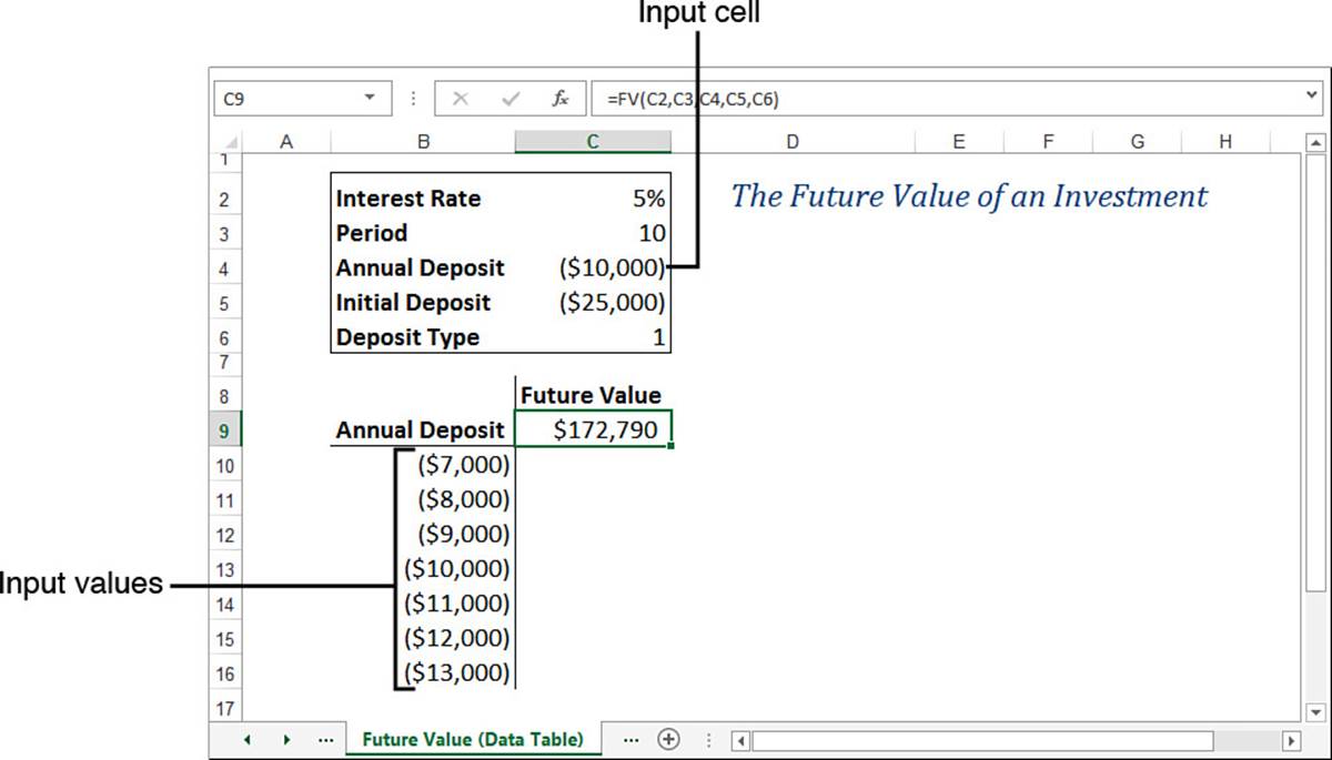
Figure 15.2 Enter the values you want to input into the formula.
2. Select the range that includes the input values and the formula. (In Figure 15.2, this is B9:C16.)
3. Select Data, What-If Analysis, Data Table. Excel displays the Data Table dialog box.
4. Fill in this dialog box based on how you set up your data table:
• If you entered the input values in a row, use the Row Input Cell text box to enter the cell address of the input cell.
• If the input values are in a column, enter the input cell’s address in the Column Input Cell text box. In the investment analysis example, you click cell C4 and then $C$4 appears in the Column Input Cell text box, as shown in Figure 15.3.
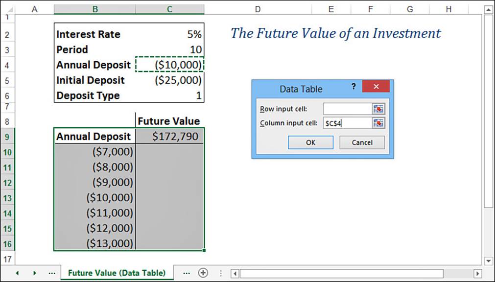
Figure 15.3 In the Data Table dialog box, enter the input cell where you want Excel to substitute the input values.
5. Click OK. Excel places each of the input values in the input cell; Excel then displays the results in the data table. Format the cells as necessary (see Figure 15.4).
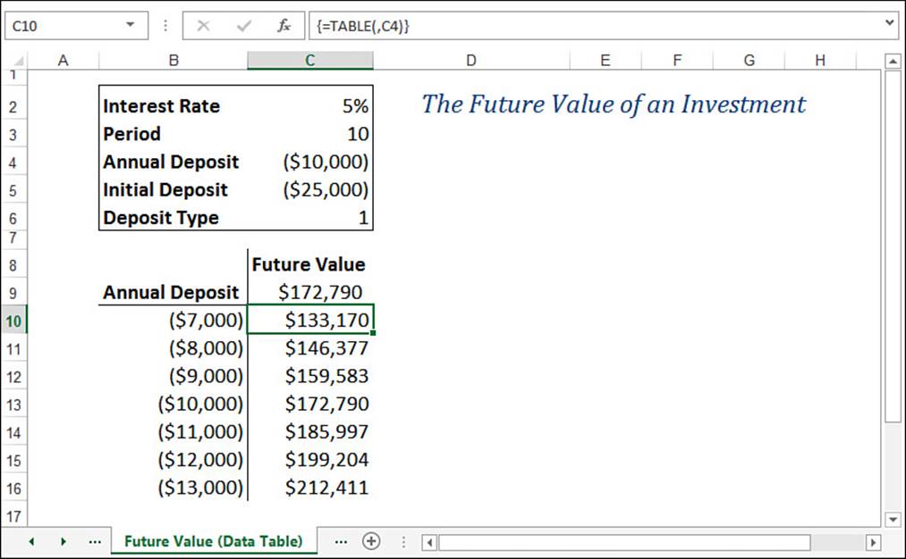
Figure 15.4 Excel substitutes each input value into the input cell and displays the results in the data table.
Adding More Formulas to the Input Table
You’re not restricted to using just a single formula in a data table. If you want to see the effect of the various input values on different formulas, you can easily add them to the data table. For example, in the future value worksheet, it would be interesting to factor inflation into the calculations to see how the investment appears in today’s dollars. Figure 15.5 shows the revised worksheet with a new Inflation variable (cell C7) and a formula that converts the calculated future value into today’s dollars (cell D9).
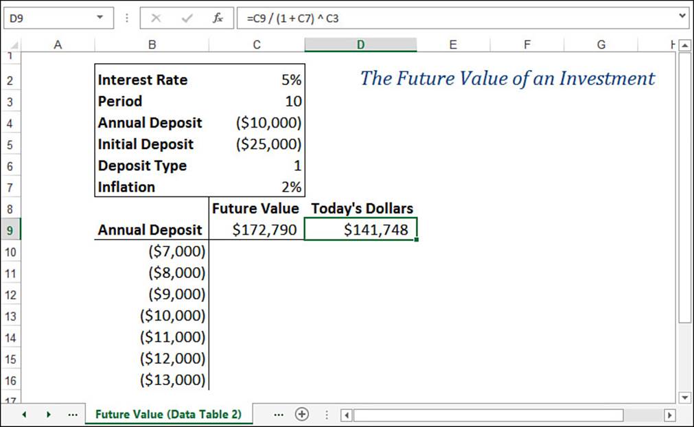
Figure 15.5 To add a formula to a data table, enter the new formula next to the existing one.
Note
This is the formula for converting a future value into today’s dollars:
Future Value / (1 + Inflation Rate) ^ Period
Here, Period is the number of years from now that the future value exists.
To create the new data table, follow the steps outlined previously. However, make sure that the range you select in step 2 includes the input values and both formulas (that is, the range B9:D16 in Figure 15.5). Figure 15.6 shows the results.
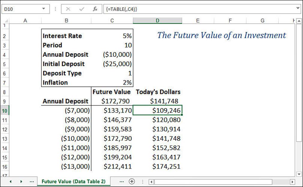
Figure 15.6 The results of using multiple formulas in the data table.
Note
After you have a data table set up, you can do regular what-if analysis by adjusting the other worksheet variables. Each time you make a change, Excel recalculates every formula in the table.
Setting Up a Two-Input Data Table
You also can set up data tables that take two input variables. This option enables you to see the effect on an investment’s future value when you enter different values—for example, the annual deposit and the interest rate. The following steps show you how to set up a two-input data table:
1. Enter one set of values in a column below the formula and the second set of values to the right of the formula in the same row, as shown in Figure 15.7.
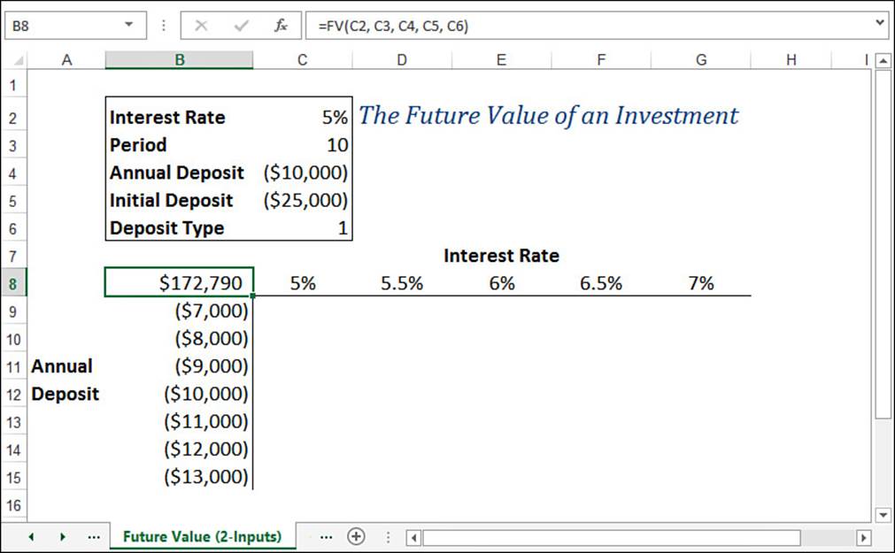
Figure 15.7 Enter the two sets of values that you want to input into the formula.
2. Select the range that includes the input values and the formula (B8:G15 in Figure 15.7).
3. Select Data, What-If Analysis, Data Table to display the Data Table dialog box.
4. In the Row Input Cell text box, enter the cell address of the input cell that corresponds to the row values you entered (C2 in Figure 15.7—the Interest Rate variable).
5. In the Column Input Cell text box, enter the cell address of the input cell you want to use for the column values (C4 in Figure 15.7—the Annual Deposit variable).
6. Click OK. Excel runs through the various input combinations and then displays the results in the data table. Format the cells as necessary (see Figure 15.8).
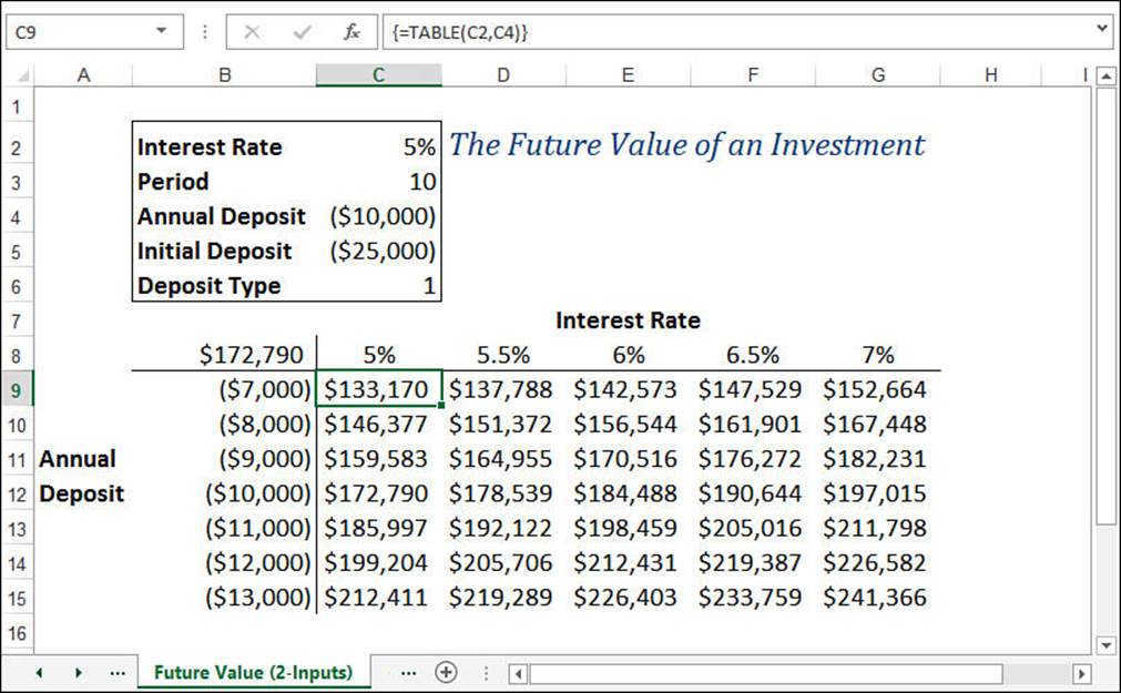
Figure 15.8 Excel substitutes each input value into the input cell and displays the results in the two-input data table.
Tip
As mentioned earlier, if you make changes to any of the variables in a table formula, Excel recalculates the entire table. This isn’t a problem in small tables, but large ones can take a very long time to calculate. If you prefer to control the table recalculation, select Formulas, Calculation, Calculation Options, Automatic Except for Data Tables. This tells Excel not to include data tables when it recalculates a worksheet. To recalculate your data tables, select Formulas, Calculation, Calculate Now (or press F9); to recalculate just the data tables in the current worksheet, select Formulas, Calculation, Calculate Sheet (or press Shift+F9).
Editing a Data Table
If you want to make changes to a data table, you can edit the formula (or formulas) as well as the input value. However, the data table results are a different matter. When you run the Data Table command, Excel enters an array formula in the interior of the data table. This formula is aTABLE() function (a special function available only by using the Data Table command) with the following syntax:
{=TABLE(row_input_ref, column_input_ref)}
Here, row_input_ref and column_input_ref are the cell references you entered in the Data Table dialog box. The braces ({ }) indicate that this is an array, which means that you can’t change or delete individual elements of the array. If you want to change the results, you need to select the entire data table and then run the Data Table command again. If you just want to delete the results, you must first select the entire array and then delete it.
![]() To learn more about arrays, see “Working with Arrays,” p. 87.
To learn more about arrays, see “Working with Arrays,” p. 87.
Working with Goal Seek
Here’s a what-if question for you: What if you already know the result you want? For example, you might know that you want to have $50,000 saved to purchase new equipment five years from now or that you have to achieve a 30% gross margin in your next budget. If you need to manipulate only a single variable to achieve these results, you can use Excel’s Goal Seek feature. You tell Goal Seek the final value you need and which variable to change, and it finds a solution for you (if one exists).
![]() For more complicated scenarios with multiple variables and constraints, you need to use Excel’s Solver feature. See Chapter 17, “Solving Complex Problems with Solver,” p. 411.
For more complicated scenarios with multiple variables and constraints, you need to use Excel’s Solver feature. See Chapter 17, “Solving Complex Problems with Solver,” p. 411.
How Does Goal Seek Work?
When you set up a worksheet to use Goal Seek, you usually have a formula in one cell and the formula’s variable—with an initial value—in another. (Your formula can have multiple variables, but Goal Seek enables you to manipulate only one variable at a time.) Goal Seek operates by using an iterative method to find a solution. That is, Goal Seek first tries the variable’s initial value to see whether that produces the result you want. If it doesn’t, Goal Seek tries different values until it converges on a solution.
![]() To learn more about iterative methods, see “Using Iteration and Circular References,” p. 93.
To learn more about iterative methods, see “Using Iteration and Circular References,” p. 93.
Running Goal Seek
Before you run Goal Seek, you need to set up your worksheet in a particular way. This means doing three things:
1. Set up one cell as the changing cell. This is the value that Goal Seek will iteratively manipulate to attempt to reach the goal. Enter an initial value (such as 0) into the cell.
2. Set up the other input values for the formula and make them proper initial values.
3. Create a formula for Goal Seek to use to try to reach the goal.
For example, suppose you’re a small-business owner looking to purchase new equipment worth $50,000 five years from now. Assuming your investments earn 5% annual interest, how much do you need to set aside every year to reach this goal? Figure 15.9 shows a worksheet set up to use Goal Seek:
![]() Cell C6 is the changing cell: the annual deposit into the fund (with an initial value of 0).
Cell C6 is the changing cell: the annual deposit into the fund (with an initial value of 0).
![]() The other cells (C4 and C5) are used as constants for the FV() function.
The other cells (C4 and C5) are used as constants for the FV() function.
![]() Cell C8 contains the FV() function that calculates the future value of the equipment fund. When Goal Seek is done, this cell’s value should be $50,000.
Cell C8 contains the FV() function that calculates the future value of the equipment fund. When Goal Seek is done, this cell’s value should be $50,000.
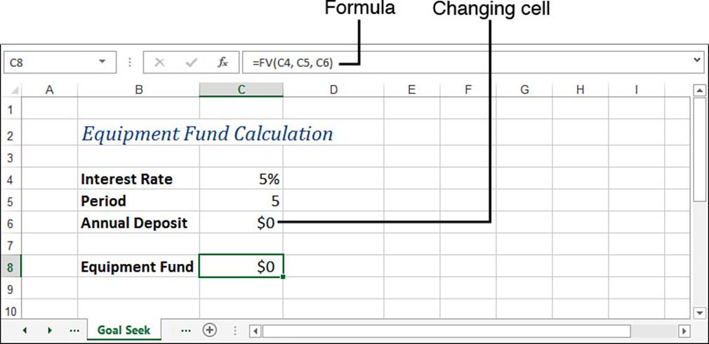
Figure 15.9 A worksheet set up to use Goal Seek to find out how much to set aside each year to end up with a $50,000 equipment fund in five years.
With your worksheet ready to go, follow these steps to use Goal Seek:
1. Select Data, What-If Analysis, Goal Seek. Excel displays the Goal Seek dialog box.
2. Use the Set Cell text box to enter a reference to the cell that contains the formula you want Goal Seek to manipulate (cell C8 in Figure 15.9).
3. Use the To Value text box to enter the final value you want for the goal cell (such as 50000).
4. Use the By Changing Cell text box to enter a reference to the changing cell. (This is cell C6 in Figure 15.9.) Figure 15.10 shows the completed Goal Seek dialog box.
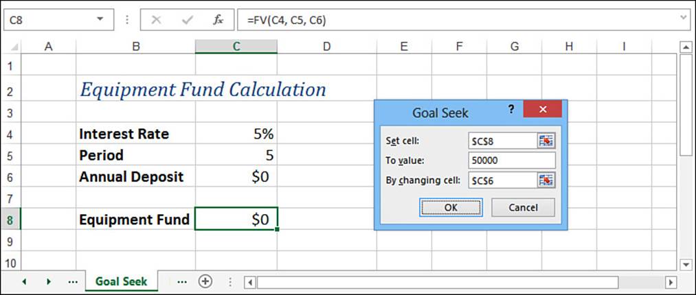
Figure 15.10 The completed Goal Seek dialog box.
5. Click OK. Excel begins the iteration and displays the Goal Seek Status dialog box. When finished, the dialog box tells you whether Goal Seek found a solution (see Figure 15.11).
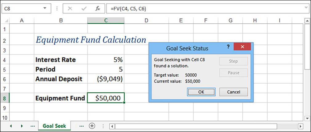
Figure 15.11 The Goal Seek Status dialog box shows you the solution (if one was found).
Note
Most of the time, Goal Seek finds a solution relatively quickly, and the Goal Seek Status dialog box displays the solution within a second or two. For longer operations, you can click Pause in the Goal Seek Status dialog box to stop Goal Seek. To walk through the process one iteration at a time, click Step. To resume Goal Seek, click Continue.
![]() You can also calculate the required annual deposit using Excel’s PMT() function; see “Calculating the Required Regular Deposit,” p. 460.
You can also calculate the required annual deposit using Excel’s PMT() function; see “Calculating the Required Regular Deposit,” p. 460.
6. If Goal Seek found a solution, you can accept the solution by clicking OK. To ignore the solution, click Cancel.
Optimizing Product Margin
Many businesses use product margin as a measure of fiscal health. A strong margin usually means that expenses are under control and that the market is satisfied with your price points. Product margin depends on many factors, of course, but you can use Goal Seek to find the optimum margin based on a single variable.
For example, suppose you want to introduce a new product line, and you want the product to return a margin of 30% during the first year. Suppose, too, that you’re operating under the following assumptions:
![]() The sales during the year will be 100,000 units.
The sales during the year will be 100,000 units.
![]() The average discount to your customers will be 40%.
The average discount to your customers will be 40%.
![]() The total fixed costs will be $750,000.
The total fixed costs will be $750,000.
![]() The cost per unit will be $12.63.
The cost per unit will be $12.63.
Given all this information, you want to know what price point will produce the 30% margin.
Figure 15.12 shows a worksheet set up to handle this situation. An initial value of $1.00 is entered into the Price per Unit cell (C4), and Goal Seek is set up in the following way:
![]() The Set Cell reference is C14, the Margin calculation.
The Set Cell reference is C14, the Margin calculation.
![]() A value of 0.3 (the 30% Margin goal) is entered in the To Value text box.
A value of 0.3 (the 30% Margin goal) is entered in the To Value text box.
![]() A reference to the Price per Unit cell (C4) is entered into the By Changing Cell text box.
A reference to the Price per Unit cell (C4) is entered into the By Changing Cell text box.
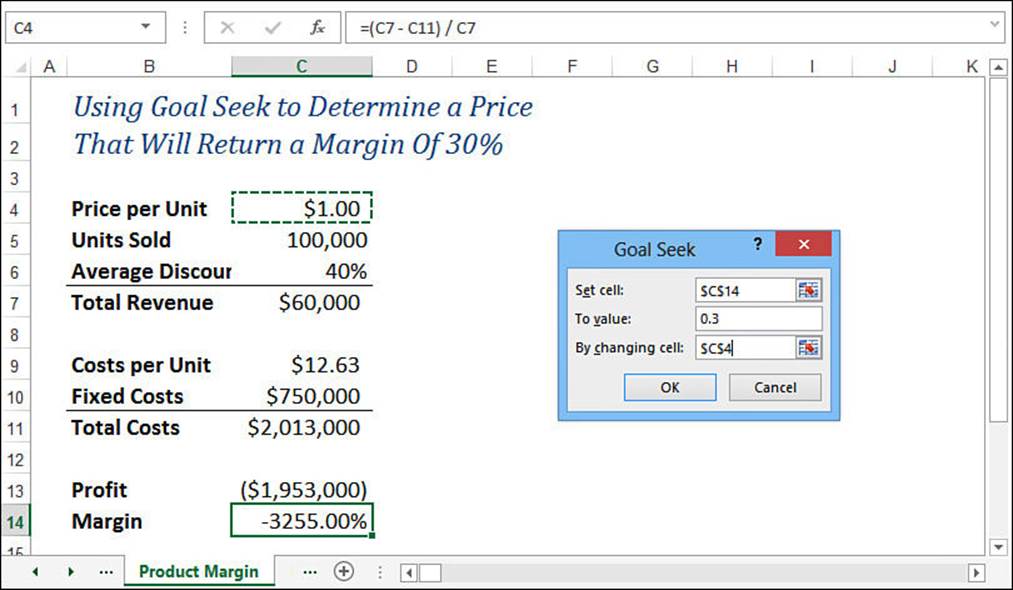
Figure 15.12 A worksheet set up to calculate a price point that will optimize gross margin.
When you run Goal Seek, it produces a solution of $47.87 for the price, as shown in Figure 15.13. This solution can be rounded up to a more standard price point of $47.95.
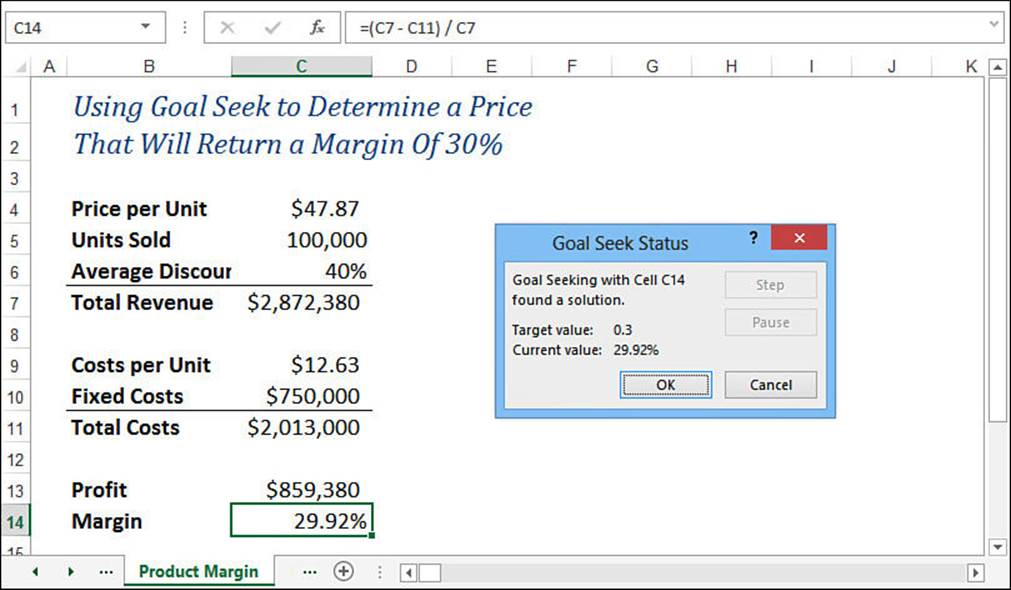
Figure 15.13 The result of Goal Seek’s labors.
A Note About Goal Seek’s Approximations
Notice that the solution in Figure 15.13 is an approximate figure. That is, the margin value is 29.92%, not the 30% you were looking for. It’s pretty close (it’s off by only 0.0008), but it’s not exact. Why didn’t Goal Seek find the exact solution?
The answer lies in one of the options Excel uses to control iterative calculations. Some iterations can take an extremely long time to find an exact solution, so Excel compromises by setting certain limits on iterative processes. To see these limits, select File, Options and then click Formulas in the Excel Options dialog box that appears (see Figure 15.14). Two options control iterative processes:
![]() Maximum Iterations—The value in this text box controls the maximum number of iterations. In Goal Seek, this represents the maximum number of values that Excel plugs into the changing cell.
Maximum Iterations—The value in this text box controls the maximum number of iterations. In Goal Seek, this represents the maximum number of values that Excel plugs into the changing cell.
![]() Maximum Change—The value in this text box is the threshold that Excel uses to determine whether it has converged on a solution. If the difference between the current solution and the desired goal is less than or equal to this value, Excel stops iterating.
Maximum Change—The value in this text box is the threshold that Excel uses to determine whether it has converged on a solution. If the difference between the current solution and the desired goal is less than or equal to this value, Excel stops iterating.
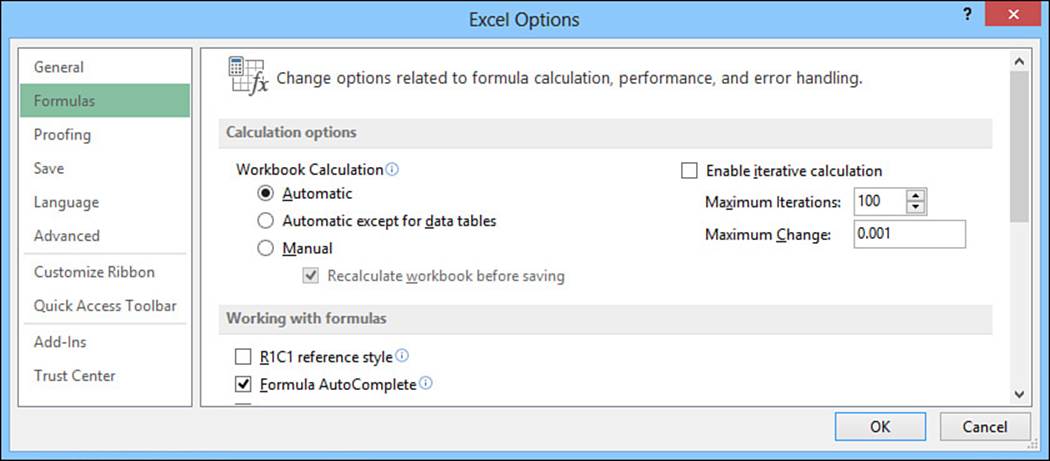
Figure 15.14 The Maximum Iterations and Maximum Change options place limits on iterative calculations.
The Maximum Change value prevented us from getting an exact solution for the profit margin calculation. On a particular iteration, Goal Seek found the solution .2992, which put us within 0.0008 of our goal of 0.3. However, 0.0008 is less than the default value of 0.001 in the Maximum Change text box, so Excel called a halt to the procedure.
To get an exact solution, you would need to adjust the Maximum Change value to 0.0001.
Performing a Break-Even Analysis
In a break-even analysis, you determine the number of units you have to sell of a product so that your total profits are 0 (that is, the product revenue equals the product costs). Setting up a profit equation with a goal of 0 and varying the units sold is perfect for Goal Seek.
To try this, we’ll extend the example used in the “Optimizing Product Margin” section. In this case, assume a unit price of $47.95 (the solution found to optimize product margin, rounded up to the nearest 95¢). Figure 15.15 shows the Goal Seek dialog box filled out as detailed here:
![]() The Set Cell reference is set to C12, the profit calculation.
The Set Cell reference is set to C12, the profit calculation.
![]() A value of 0 (the profit goal) is entered in the To Value text box.
A value of 0 (the profit goal) is entered in the To Value text box.
![]() A reference to the Units Sold cell (C4) is entered into the By Changing Cell text box.
A reference to the Units Sold cell (C4) is entered into the By Changing Cell text box.
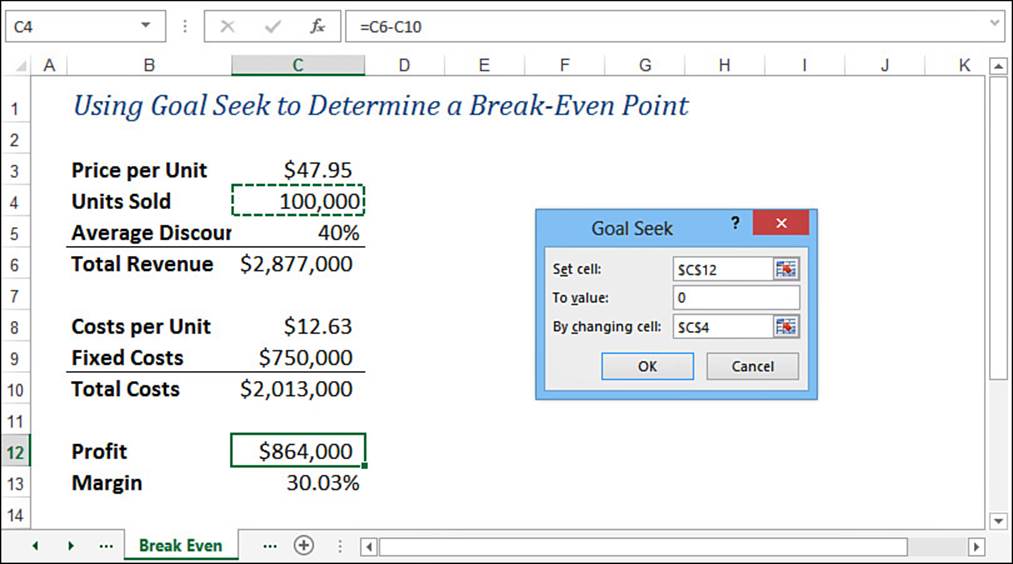
Figure 15.15 A worksheet set up to calculate a price point that optimizes gross margin.
Figure 15.16 shows the solution: A total of 46,468 units must be sold to break even.
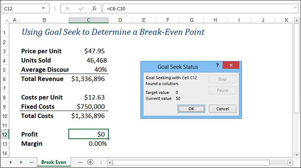
Figure 15.16 The break-even solution.
Solving Algebraic Equations
Algebraic equations don’t come up all that often in a business context, but they do appear occasionally in complex models. Fortunately, Goal Seek also is useful for solving complex algebraic equations of one variable. For example, suppose you need to find the value of x to solve the rather nasty equation displayed in Figure 15.17. Although this equation is too complex for the quadratic formula, it can be easily rendered in Excel. The left side of the equation can be represented with the following formula:
=(((3 * A2 - 8) ^ 2) * (A2 - 1)) / (4 * A2 ^ 2 - 5)
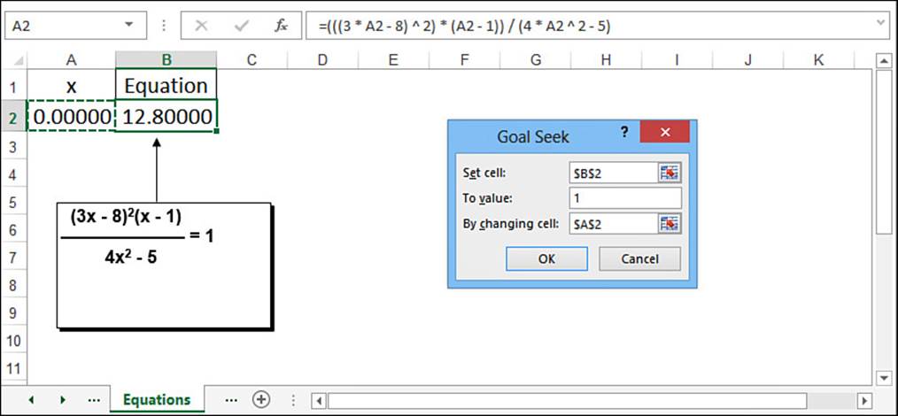
Figure 15.17 Solving an algebraic equation with Goal Seek.
Cell A2 represents the variable x. You can solve this equation in Goal Seek by setting the goal for this equation to 1 (the right side of the equation) and by varying cell A2. Figure 15.17 shows a worksheet and the Goal Seek dialog box.
Figure 15.18 shows the result. The value in cell A2 is the solution (x) that satisfies the equation. Notice that the equation result (cell B2) is not quite 1. As mentioned earlier in this chapter, if you need higher accuracy, you must change Excel’s convergence threshold. In this example, select File, Options, click Formulas, and type 0.000001 in the Maximum Change text box.
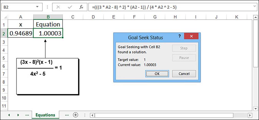
Figure 15.18 Cell A2 holds the solution for the equation in cell B2.
Working with Scenarios
By definition, what-if analysis is not an exact science. All what-if models make guesses and assumptions based on history, expected events, or some sort of voodoo. A particular set of guesses and assumptions that you plug into a model is called a scenario. Because most what-if worksheets can take a wide range of input values, you usually end up with a large number of scenarios to examine. Instead of going through the tedious chore of inserting all these values into the appropriate cells, Excel has a Scenario Manager feature that can handle the process for you. This section shows you how to wield this useful tool.
Understanding Scenarios
As you’ve seen in this chapter, Excel has powerful features that enable you to build sophisticated models that can answer complex questions. The problem, though, isn’t in answering questions, but in asking them. For example, Figure 15.19 shows a worksheet model that analyzes a mortgage. You use this model to decide how much of a down payment to make, how long the term should be, and whether to include an extra principal paydown every month. The Results section compares the monthly payment and total paid for the regular mortgage and for the mortgage with a paydown. It also shows the savings and reduced term that result from the paydown.
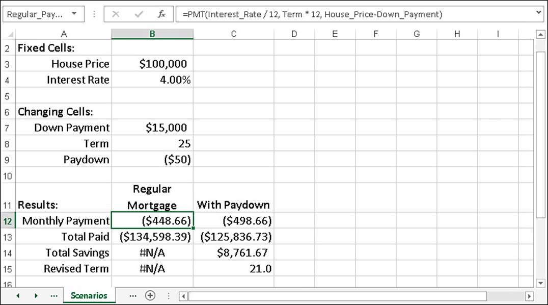
Figure 15.19 A mortgage analysis worksheet.
![]() The formula shown in Figure 15.19 uses the PMT() function, which is covered later in the book; see “Calculating a Loan Payment,” p. 435.
The formula shown in Figure 15.19 uses the PMT() function, which is covered later in the book; see “Calculating a Loan Payment,” p. 435.
Here are some possible questions to ask this model:
![]() How much will I save over the term of the mortgage if I use a shorter term, make a larger down payment, and include a monthly paydown?
How much will I save over the term of the mortgage if I use a shorter term, make a larger down payment, and include a monthly paydown?
![]() How much more will I end up paying if I extend the term, reduce the down payment, and forgo the paydown?
How much more will I end up paying if I extend the term, reduce the down payment, and forgo the paydown?
These are examples of scenarios that you would plug into the appropriate cells in the model. Excel’s Scenario Manager helps by letting you define a scenario separately from the worksheet. You can save specific values for any or all of the model’s input cells, give the scenario a name, and then recall the name (and all the input values it contains) from a list.
Setting Up Your Worksheet for Scenarios
Before creating a scenario, you need to decide which cells in your model will be the input cells. These will be the worksheet variables—the cells that, when you change them, change the results of the model. (Not surprisingly, Excel calls these the changing cells.) You can have as many as 32 changing cells in a scenario. For best results, follow these guidelines when setting up your worksheet for scenarios:
![]() The changing cells should be constants. Formulas can be affected by other cells, and that can throw off the entire scenario.
The changing cells should be constants. Formulas can be affected by other cells, and that can throw off the entire scenario.
![]() To make it easier to set up each scenario and to make your worksheet easier to understand, group the changing cells and label them (see Figure 15.19).
To make it easier to set up each scenario and to make your worksheet easier to understand, group the changing cells and label them (see Figure 15.19).
![]() For even greater clarity, assign a range name to each changing cell.
For even greater clarity, assign a range name to each changing cell.
Adding a Scenario
To work with scenarios, you use Excel’s Scenario Manager tool. This feature enables you to add, edit, display, and delete scenarios as well as create summary scenario reports.
When your worksheet is set up the way you want it, you can add a scenario to the sheet by following these steps:
1. Select Data, What-If Analysis, Scenario Manager. Excel displays the Scenario Manager dialog box, shown in Figure 15.20.
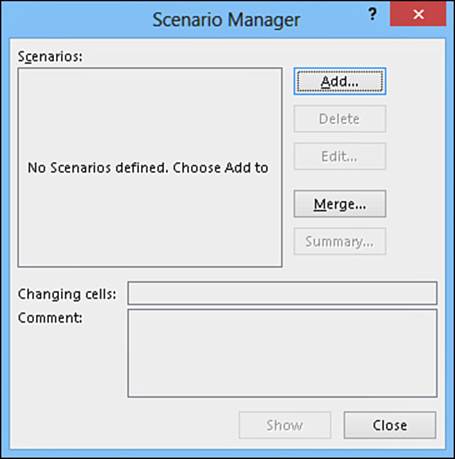
Figure 15.20 Excel’s Scenario Manager enables you to create and work with worksheet scenarios.
2. Click Add. The Add Scenario dialog box appears. Figure 15.21 shows a completed version of this dialog box.
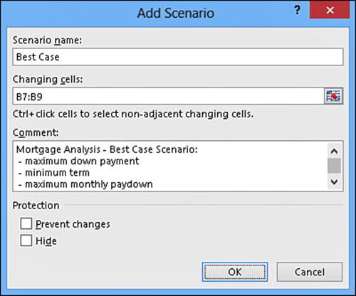
Figure 15.21 Use the Add Scenario dialog box to define a scenario.
3. Use the Scenario Name text box to enter a name for the scenario.
4. Use the Changing Cells box to enter references to your worksheet’s changing cells. You can type in the references (be sure to separate noncontiguous cells with commas) or select the cells directly on the worksheet.
5. Use the Comment box to enter a description for the scenario. This description appears in the Comment section of the Scenario Manager dialog box.
6. Click OK. Excel displays the Scenario Values dialog box, shown in Figure 15.22.
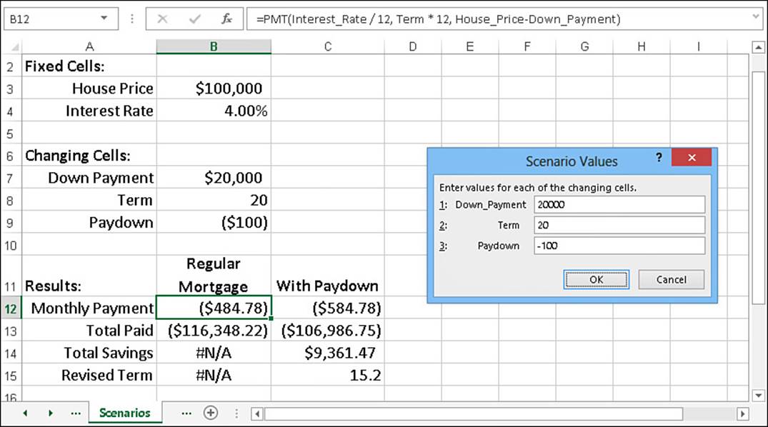
Figure 15.22 Use the Scenario Values dialog box to enter the values you want to use for the scenario’s changing cells.
7. Use the text boxes to enter values for the changing cells.
Note
Notice in Figure 15.22 that Excel displays the range name for each changing cell, which makes it easier to enter your numbers correctly. If your changing cells aren’t named, Excel just displays the cell addresses instead.
8. To add more scenarios, click Add to return to the Add Scenario dialog box and repeat steps 3 through 7. Otherwise, click OK to return to the Scenario Manager dialog box.
9. Click Close to return to the worksheet.
Displaying a Scenario
After you define a scenario, you can enter its values into the changing cells by displaying the scenario from the Scenario Manager dialog box. The following steps give you the details:
1. Select Data, What-If Analysis, Scenario Manager.
2. In the Scenarios list, click the scenario you want to display.
3. Click Show. Excel enters the scenario values into the changing cells. Figure 15.23 shows an example.
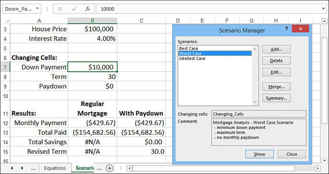
Figure 15.23 When you click Show, Excel enters the values for the highlighted scenario into the changing cells.
4. Repeat steps 2 and 3 to display other scenarios.
5. Click Close to return to the worksheet.
Tip
Displaying a scenario isn’t hard, but it does require having the Scenario Manager onscreen. You can bypass the Scenario Manager by adding the Scenario list to the Quick Access Toolbar. Pull down the Customize Quick Access Toolbar menu and then click More Commands. In the Choose Commands From list, click All Commands. In the list of commands, click Scenario, click Add, and then click OK. (One caveat, though: If you select the same scenario twice in succession, Excel asks whether you want to redefine the scenario. Be sure to click No to keep the current scenario definition.)
Editing a Scenario
If you need to make changes to a scenario—whether to change the scenario’s name, select different changing cells, or enter new values—follow these steps:
1. Select Data, What-If Analysis, Scenario Manager.
2. In the Scenarios list, click the scenario you want to edit.
3. Click Edit. Excel displays the Edit Scenario dialog box (which is identical to the Add Scenario dialog box, shown in Figure 15.21).
4. Make your changes, if necessary, and click OK. The Scenario Values dialog box appears (refer to Figure 15.22).
5. Enter the new values, if necessary, and then click OK to return to the Scenario Manager dialog box.
6. Repeat steps 2 through 5 to edit other scenarios.
7. Click Close to return to the worksheet.
Merging Scenarios
The scenarios you create are stored with each worksheet in a workbook. If you have similar models in different sheets (for example, budget models for different divisions), you can create separate scenarios for each sheet and then merge them later. Here are the steps to follow:
1. Select the worksheet in which you want to store the merged scenarios.
2. Select Data, What-If Analysis, Scenario Manager.
3. Click Merge. Excel displays the Merge Scenarios dialog box, shown in Figure 15.24.
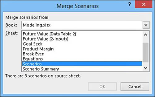
Figure 15.24 Use the Merge Scenarios dialog box to select the scenarios you want to merge.
4. Use the Book drop-down list to click the workbook that contains the scenario sheet.
5. Use the Sheet list to click the worksheet that contains the scenario.
6. Click OK to return to the Scenario Manager.
7. Click Close to return to the worksheet.
Generating a Summary Report
You can create a summary report that shows the changing cells in each of your scenarios along with selected result cells. This is a handy way to compare different scenarios. You can try it by following these steps:
Note
When Excel sets up the scenario summary, it uses either the cell addresses or defined names of the individual changing cells and results cells, as well as the entire range of changing cells. Your reports will be more readable if you name the cells you’ll be using before generating the summary.
1. Select Data, What-If Analysis, Scenario Manager.
2. Click Summary. Excel displays the Scenario Summary dialog box.
3. In the Report Type group, click either Scenario Summary or Scenario PivotTable Report.
4. In the Result Cells box, enter references to the result cells that you want to appear in the report (see Figure 15.25). You can select the cells directly on the sheet or type in the references. (Remember to separate noncontiguous cells with commas.)
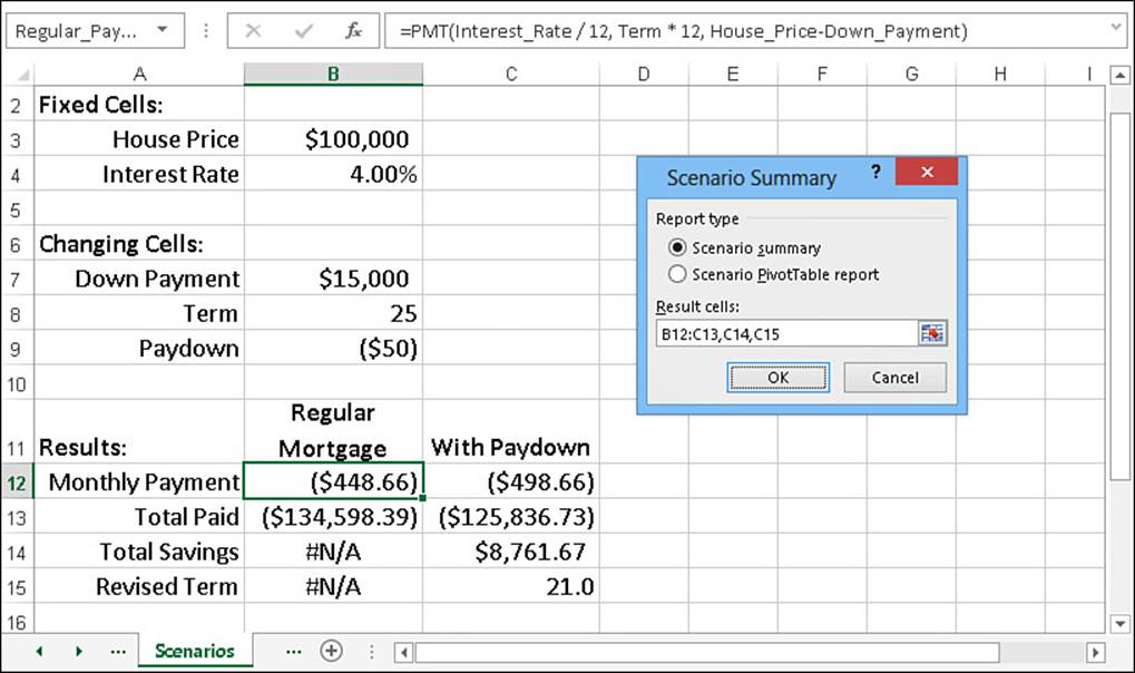
Figure 15.25 Use the Scenario Summary dialog box to select the report type and result cells.
5. Click OK. Excel displays the report.
Figure 15.26 shows the Scenario Summary report for the Mortgage Analysis worksheet. The names shown in column C (Down_Payment, Term, and so on) are the names I assigned to each of the changing cells and result cells.
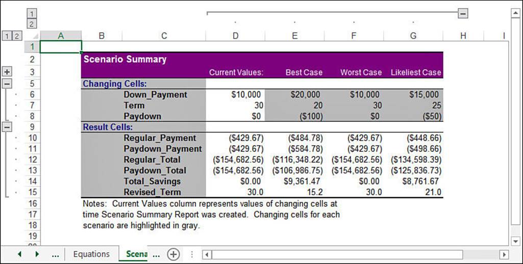
Figure 15.26 The Scenario Summary report for the Mortgage Analysis worksheet.
Figure 15.27 shows the Scenario PivotTable report for the Mortgage Analysis worksheet.
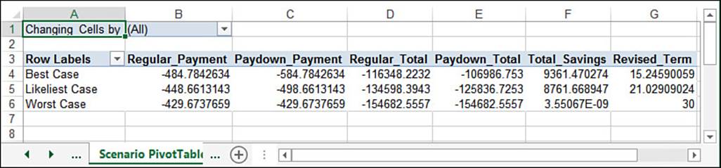
Figure 15.27 The Scenario PivotTable report for the Mortgage Analysis worksheet.
Note
The PivotTable’s page field—labeled Changing Cells By—enables you to switch between scenarios created by different users. If no other users have access to this workbook, you’ll see only your name in this field’s list.
Deleting a Scenario
If you have scenarios you no longer need, you can delete them by following these steps:
1. Select Data, What-If Analysis, Scenario Manager.
2. Use the Scenarios list to click the scenario you want to delete.
Caution
Excel doesn’t ask you to confirm the deletion, and there’s no way to retrieve a scenario that has been deleted accidentally (other than closing the workbook without saving changes or opening a previous version of the workbook), so be sure the scenario you highlighted is one you can live without.
3. Click Delete. Excel deletes the scenario.
4. Click Close to return to the worksheet.
From Here
![]() To understand and use iterative methods, see “Using Iteration and Circular References,” p. 93.
To understand and use iterative methods, see “Using Iteration and Circular References,” p. 93.
![]() Consolidating data is useful for analyzing models that have similar data spread out over multiple sheets. To learn how this is done, see “Consolidating Multisheet Data,” p. 95.
Consolidating data is useful for analyzing models that have similar data spread out over multiple sheets. To learn how this is done, see “Consolidating Multisheet Data,” p. 95.
![]() Goal Seek’s “big brother” is the Solver tool. See Chapter 17, “Solving Complex Problems with Solver,” p. 411.
Goal Seek’s “big brother” is the Solver tool. See Chapter 17, “Solving Complex Problems with Solver,” p. 411.
![]() Excel’s Solver tool enables you to save its solutions as scenarios. See “Saving a Solution as a Scenario,” p. 418.
Excel’s Solver tool enables you to save its solutions as scenarios. See “Saving a Solution as a Scenario,” p. 418.
![]() For the details of the PMT() function from a loan perspective, see “Calculating the Loan Payment,” p. 435.
For the details of the PMT() function from a loan perspective, see “Calculating the Loan Payment,” p. 435.
![]() To learn how to use PMT() to calculate the deposits required to reach an investment goal, see “Calculating the Required Regular Deposit,” p. 460.
To learn how to use PMT() to calculate the deposits required to reach an investment goal, see “Calculating the Required Regular Deposit,” p. 460.
All materials on the site are licensed Creative Commons Attribution-Sharealike 3.0 Unported CC BY-SA 3.0 & GNU Free Documentation License (GFDL)
If you are the copyright holder of any material contained on our site and intend to remove it, please contact our site administrator for approval.
© 2016-2026 All site design rights belong to S.Y.A.