Excel® 2016 Formulas and Functions (2016)
Part III: Building Business Models
17. Solving Complex Problems with Solver
In This Chapter
Some Background on Solver
Loading Solver
Using Solver
Adding Constraints
Saving a Solution as a Scenario
Setting Other Solver Options
Making Sense of Solver’s Messages
Displaying Solver’s Reports
In Chapter 15, “Using Excel’s Business Modeling Tools,” you learned how to use Goal Seek to find solutions to formulas by changing a single variable. Unfortunately, most problems in business aren’t so easy. You’ll usually face formulas with at least two and sometimes dozens of variables. Often, a problem will have more than one solution, and your challenge will be to find the optimal solution (that is, the one that maximizes profit, or minimizes costs, or matches other criteria). For these bigger challenges, you need a more muscular tool. Excel has just the answer: Solver. Solver is a sophisticated optimization program that enables you to find solutions to complex problems that would otherwise require high-level mathematical analysis. This chapter introduces you to Solver (a complete discussion would require a book in itself) and takes you through a few examples.
Some Background on Solver
Problems such as “What product mix will maximize profit?” and “What transportation routes will minimize shipping costs while meeting demand?” traditionally have been solved by using numerical methods such as linear programming and nonlinear programming. An entire mathematical field known as operations research has been developed to handle such problems, which are found in all kinds of disciplines. The drawback to linear and nonlinear programming is that solving even the simplest problem by hand is a complicated, arcane, and time-consuming business. In other words, it’s a perfect job to hand off to a computer.
This is where Solver comes in. Solver incorporates many of the algorithms from operations research, but it keeps the sordid details in the background. All you do is fill out a dialog box or two, and Solver does the rest.
The Advantages of Solver
Solver, like Goal Seek, uses an iterative method to perform its magic. This means that Solver tries a solution, analyzes the results, tries another solution, and so on. However, this cyclic iteration isn’t just guesswork on Solver’s part. The program looks at how the results change with each new iteration and, through some sophisticated mathematical trickery, can tell (usually) in what direction it should head for the solution.
However, the fact that Goal Seek and Solver are both iterative doesn’t make them equal. In fact, Solver brings a number of advantages to the table:
![]() Solver enables you to specify multiple adjustable cells. You can use up to 200 adjustable cells in all.
Solver enables you to specify multiple adjustable cells. You can use up to 200 adjustable cells in all.
![]() Solver enables you to set up constraints on the adjustable cells. For example, you can tell Solver to find a solution that not only maximizes profit but also satisfies certain conditions, such as achieving a gross margin between 20% and 30%, or keeping expenses less than $100,000. These conditions are said to be constraints on the solution.
Solver enables you to set up constraints on the adjustable cells. For example, you can tell Solver to find a solution that not only maximizes profit but also satisfies certain conditions, such as achieving a gross margin between 20% and 30%, or keeping expenses less than $100,000. These conditions are said to be constraints on the solution.
![]() Solver seeks not only a desired result (the “goal” in Goal Seek), but also the optimal one. This means you can find a solution that is the maximum or minimum possible.
Solver seeks not only a desired result (the “goal” in Goal Seek), but also the optimal one. This means you can find a solution that is the maximum or minimum possible.
![]() For complex problems, Solver can generate multiple solutions. You then can save these different solutions under different scenarios, as described later in this chapter.
For complex problems, Solver can generate multiple solutions. You then can save these different solutions under different scenarios, as described later in this chapter.
When Do You Use Solver?
Solver is a powerful tool that most Excel users don’t need. It would be overkill, for example, to use Solver to compute net profit given fixed revenue and cost figures. Many problems, however, require nothing less than the Solver approach. These problems cover many different fields and situations, but they all have the following characteristics in common:
![]() They have a single objective cell (also called the target cell) that contains a formula you want to maximize, minimize, or set to a specific value. This formula could be a calculation, such as total transportation expenses or net profit.
They have a single objective cell (also called the target cell) that contains a formula you want to maximize, minimize, or set to a specific value. This formula could be a calculation, such as total transportation expenses or net profit.
![]() The objective cell formula contains references to one or more variable cells (also called unknowns or changing cells). Solver adjusts these cells to find the optimal solution for the objective cell formula. These variable cells might include items such as units sold, shipping costs, or advertising expenses.
The objective cell formula contains references to one or more variable cells (also called unknowns or changing cells). Solver adjusts these cells to find the optimal solution for the objective cell formula. These variable cells might include items such as units sold, shipping costs, or advertising expenses.
![]() Optionally, there are one or more constraint cells that must satisfy certain criteria. For example, you might require that advertising be less than 10% of total expenses, or that the discount to customers be a number between 40% and 60%.
Optionally, there are one or more constraint cells that must satisfy certain criteria. For example, you might require that advertising be less than 10% of total expenses, or that the discount to customers be a number between 40% and 60%.
What types of problems exhibit these kinds of characteristics? A surprisingly broad range, as the following list shows:
![]() The transportation problem—This problem involves minimizing shipping costs from multiple manufacturing plants to multiple warehouses, while meeting demand.
The transportation problem—This problem involves minimizing shipping costs from multiple manufacturing plants to multiple warehouses, while meeting demand.
![]() The allocation problem—This problem requires minimizing employee costs while maintaining appropriate staffing requirements.
The allocation problem—This problem requires minimizing employee costs while maintaining appropriate staffing requirements.
![]() The product mix problem—This problem requires generating the maximum profit with a mix of products while still meeting customer requirements. You solve this problem when you sell multiple products with different cost structures, profit margins, and demand curves.
The product mix problem—This problem requires generating the maximum profit with a mix of products while still meeting customer requirements. You solve this problem when you sell multiple products with different cost structures, profit margins, and demand curves.
![]() The blending problem—This problem involves manipulating the materials used for one or more products to minimize production costs, meet consumer demand, and maintain a minimum level of quality.
The blending problem—This problem involves manipulating the materials used for one or more products to minimize production costs, meet consumer demand, and maintain a minimum level of quality.
![]() Linear algebra—This problem involves solving sets of linear equations.
Linear algebra—This problem involves solving sets of linear equations.
Loading Solver
Solver is an add-in to Microsoft Excel, so you need to load Solver before you can use it. Follow these steps to load Solver:
1. Select File, Options to open the Excel Options dialog box.
2. Click Add-Ins.
3. Use the Manage list to click Excel Add-Ins and then click Go. Excel displays the Add-Ins dialog box.
4. In the Add-Ins Available list, click to select the Solver Add-In check box.
5. Click OK.
6. If Solver isn’t installed, Excel displays a dialog box to let you know. Click Yes. Excel installs the add-in and adds a Solver button to the Data tab’s Analyze group.
Using Solver
To help you get a feel for how Solver works, let’s look at an example. In Chapter 15, you used Goal Seek to compute the break-even point for a new product. (Recall that the break-even point is the number of units that need to be sold to produce a profit of 0.) I’ll extend this analysis by computing the break-even point for two products: a Finley sprocket and a Langstrom wrench. The goal is to compute the number of units to sell for both products so that the total profit is 0.
The most obvious way to proceed is to run Goal Seek twice to determine the break-even points for each product separately. Figure 17.1 shows the results.
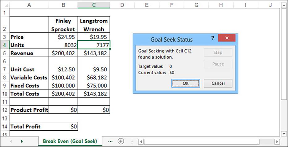
Figure 17.1 The break-even points for two products (using separate Goal Seek calculations on the Product Profit cells).
Note
You can download this chapter’s sample workbook at www.mcfedries.com/books/book.php?title=excel-2016-formulas-and-functions.
This method works, but the problem is that the two products don’t exist in a vacuum. For example, there will be cost savings associated with each product because of joint advertising campaigns, combined shipments to customers (larger shipments usually mean better freight rates), and so on. To allow for this, you need to reduce the cost for each product by a factor related to the number of units sold of the other product. In practice, this would be difficult to estimate, but to keep things simple, I’ll use the following assumption: The costs for each product are reduced by $1 for every unit sold of the other product. For instance, if the Langstrom wrench sells 10,000 units, the costs for the Finley sprocket are reduced by $10,000. I’ll make this adjustment in the Variable Costs formula. For example, the formula that calculates variable costs for the Finley sprocket (cell B8) becomes the following:
=B4 * B7 - C4
Similarly, the formula that calculates variable costs for the Langstrom wrench (cell C8) becomes the following:
=C4 * C7 - B4
By making this change, you move out of Goal Seek’s territory. The Variable Costs formulas now have two variables: the units sold for the Finley sprocket and the units sold for the Langstrom wrench. I’ve changed the problem from one of two single-variable formulas, which Goal Seek can easily handle (individually), to a single formula with two variables, which is the terrain of Solver.
To see how Solver handles such a problem, follow these steps:
1. Select Data, Solver. Excel displays the Solver Parameters dialog box.
2. In the Set Objective range box, enter a reference to the objective cell—that is, the cell with the formula you want to optimize. In the example, you enter B14. (Note that Solver converts your relative references to absolute references.)
3. In the To section, select the appropriate option button: Click Max to maximize the objective cell, click Min to minimize it, or click Value Of to solve for a particular value (in which case you also need to enter the value in the text box provided). In the example, you click Value Of and enter 0 in the text box.
4. Use the By Changing Variable Cells box to enter the cells you want Solver to change while it looks for a solution. In the example, you enter B4,C4. Figure 17.2 shows the completed Solver Parameters dialog box for this example. (Note that Solver changes all cell addresses to the absolute reference format.)
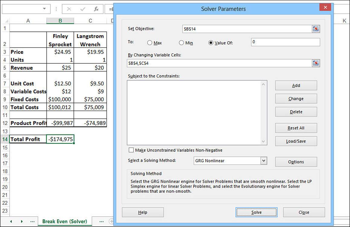
Figure 17.2 Use the Solver Parameters dialog box to set up the problem for Solver.
Note
You can enter a maximum of 200 cells in the By Changing Variable Cells text box.
5. Click Solve. (I discuss constraints and other Solver options in the next few sections.) As Solver works on the problem, you might see one or more Show Trial Solution dialog boxes. If so, click Continue in each one. Finally, Solver displays the Solver Results dialog box, which tells you whether it found a solution. (See the section “Making Sense of Solver’s Messages,” later in this chapter.)
6. If Solver found a solution you want to use, click the Keep Solver Solution option and then click OK. If you don’t want to accept the new numbers, click Restore Original Values and click OK or just click Cancel. (To learn how to save a solution as a scenario, see the section “Saving a Solution as a Scenario,” later in this chapter.)
Figure 17.3 shows the results for this example. As you can see, Solver has produced a total profit of 0 by running one product (the Langstrom wrench) at a slight loss and the other at a slight profit. Although this is certainly a solution, it’s not really the one you want. Ideally, for a true break-even analysis, both products should end up with a product profit of 0. The problem is that you didn’t tell Solver that was the way you wanted the problem solved. In other words, you didn’t set up any constraints.
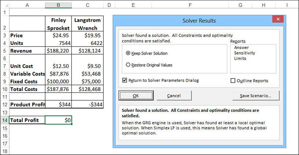
Figure 17.3 When Solver finishes its calculations, it displays the Solver Results dialog box and enters the solution (if it found one) into the worksheet cells.
Adding Constraints
The real world puts restrictions and conditions on formulas. A factory might have a maximum capacity of 10,000 units a day, the number of employees in a company has to be a number greater than or equal to zero (negative employees would really reduce staff costs, but nobody has been able to figure out how to do it yet), and your advertising costs might be restricted to 10% of total expenses. These are examples of what Solver calls constraints. Adding constraints tells Solver to find a solution so that these conditions are not violated.
To find the best solution for the break-even analysis, you need to tell Solver to optimize both Product Profit formulas to 0. The following steps show you how to do this:
Note
If Solver’s completion message is still onscreen from the last section, select Cancel to return to the worksheet without saving the solution.
1. Select Data, Solver to display the Solver Parameters dialog box. Solver reinstates the options you entered the last time you used Solver.
2. To add a constraint, click Add. Excel displays the Add Constraint dialog box.
3. In the Cell Reference box, enter the cell you want to constrain. In this case, enter cell B12 (the Product Profit formula for the Finley sprocket).
4. Use the drop-down list in the middle of the dialog box to select the operator you want to use. The list contains several comparison operators for the constraint—less than or equal to (<=), equal to (=), and greater than or equal to (>=)—as well as two other data type operators—integer (int) and binary (bin). In this case, select the equal to operator (=).
Note
Use the int (integer) operator when you need a constraint, such as total employees, to be an integer value instead of a real number. Use the bin (binary) operator when you have a constraint that must be either TRUE or FALSE (or 1 or 0).
5. If you chose a comparison operator in step 4, use the Constraint box to enter the value by which you want to restrict the cell. In this case, enter 0. Figure 17.4 shows the completed dialog box for this example.
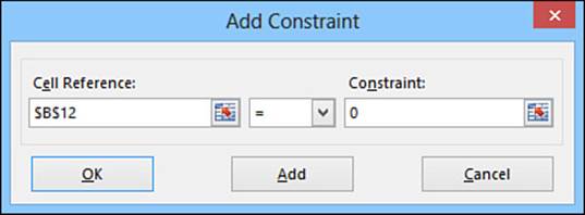
Figure 17.4 Use the Add Constraint dialog box to specify the constraints you want to place on the solution.
6. If you want to enter more constraints, click Add and repeat steps 3 through 5. For the example, you also need to constrain cell C12 (the Product Profit formula for the Langstrom wrench) so that it, too, equals 0.
7. When you’re done, click OK to return to the Solver Parameters dialog box. Excel displays your constraints in the Subject to the Constraints list box.
Note
You can add a maximum of 100 constraints. Also, if you need to make a change to a constraint before you begin solving, click the constraint in the Subject to the Constraints list box, click Change, and then make your adjustments in the Change Constraint dialog box that appears. If you want to delete a constraint that you no longer need, click it and then click Delete.
8. Click Solve. Solver again tries to find a solution, but this time it uses your constraints as guidelines. Note that you might need to click Continue one or more times while Solver works on the solution.
Figure 17.5 shows the results of the break-even analysis after the constraints have been added. As you can see, Solver was able to find a solution in which both product margins are 0.
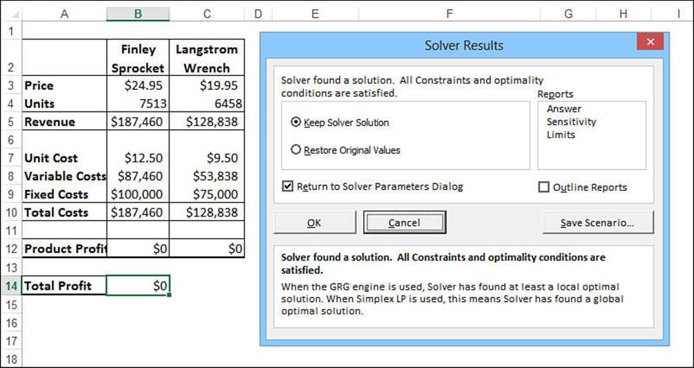
Figure 17.5 The solution to the break-even analysis after the constraints have been added.
Saving a Solution as a Scenario
If Solver finds a solution, you can save the variable cells as a scenario that you can display at any time. Use the following steps to save a solution as a scenario:
1. Select Data, Solver to display the Solver Parameters dialog box.
2. Enter the appropriate objective cell, variable cells, and constraints, if necessary.
3. Click Solve to begin solving.
4. If Solver finds a solution, click Save Scenario in the Solver Results dialog box. Excel displays the Save Scenario dialog box.
5. Use the Scenario Name text box to enter a name for the scenario.
6. Click OK. Excel returns you to the Solver Results dialog box.
7. Keep or discard the solution, as appropriate.
![]() To learn about scenarios, see “Working with Scenarios,” p. 362.
To learn about scenarios, see “Working with Scenarios,” p. 362.
Setting Other Solver Options
Most Solver problems should respond to the basic objective-cell/variable-cell/constraint-cell model you’ve looked at so far. However, for times when you’re having trouble getting a solution for a particular model, Solver has a number of options that might help. Start Solver and, in the Solver Parameters dialog box, first note the check box named Make Unconstrained Variables Non-Negative. Select this check box to force Solver to assume that the cells listed in the By Changing Variable Cells list must have values greater than or equal to 0. This is the same as adding >=0constraints for each of those cells, so it operates as a kind of implicit constraint on them. This is handy in models that use quite a few variable cells, none of which should have negative values.
Selecting the Method Solver Uses
Solver can use one of several solving methods—called engines—to perform its calculations. In the Solver Parameters dialog box, use the Select a Solving Method list to select one of the following engines:
![]() Simplex LP—Select this engine if your worksheet model is linear. In the simplest possible terms, a linear model is one in which the variables are not raised to any powers and none of the so-called transcendent functions—such as SIN() and COS()—is used. A linear model is so named because it can be charted as straight lines. If your formulas are linear, be sure to select Simplex LP because this will greatly speed up the solution process.
Simplex LP—Select this engine if your worksheet model is linear. In the simplest possible terms, a linear model is one in which the variables are not raised to any powers and none of the so-called transcendent functions—such as SIN() and COS()—is used. A linear model is so named because it can be charted as straight lines. If your formulas are linear, be sure to select Simplex LP because this will greatly speed up the solution process.
![]() GRG Nonlinear—Select this engine if your worksheet model is nonlinear and smooth. In general terms, a smooth model is one in which a graph of the equation used would show no sharp edges or breaks (called discontinuities).
GRG Nonlinear—Select this engine if your worksheet model is nonlinear and smooth. In general terms, a smooth model is one in which a graph of the equation used would show no sharp edges or breaks (called discontinuities).
![]() Evolutionary—Select this engine if your worksheet model is nonlinear and non-smooth. In practical terms, this usually means your worksheet model uses functions such as VLOOKUP(), HLOOKUP(), CHOOSE(), and IF() to calculate the values of the variable cells or constraint cells.
Evolutionary—Select this engine if your worksheet model is nonlinear and non-smooth. In practical terms, this usually means your worksheet model uses functions such as VLOOKUP(), HLOOKUP(), CHOOSE(), and IF() to calculate the values of the variable cells or constraint cells.
Note
If you’re not sure which engine to use, start with Simplex LP. If it turns out that your model is nonlinear, Solver will recognize this and let you know. You can then try the GRG Nonlinear engine; if Solver can’t seem to converge on a solution, you should try the Evolutionary engine.
Controlling How Solver Works
Solver has several options that you can set to determine how the tool performs its tasks. To see these options, open the Solver Parameters dialog box and click Options to display the Options dialog box, shown in Figure 17.6.
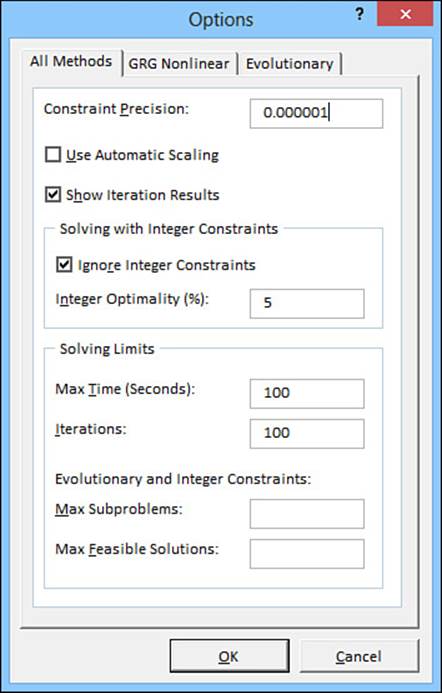
Figure 17.6 The Options dialog box controls how Solver solves a problem.
The following options in the All Methods tab control how Solver works no matter which method you use:
![]() Constraint Precision—This number determines how close a constraint cell must be to the constraint value you entered before Solver declares the constraint satisfied. The higher the precision (that is, the lower the number), the more accurate the solution but the longer it takes Solver to find it.
Constraint Precision—This number determines how close a constraint cell must be to the constraint value you entered before Solver declares the constraint satisfied. The higher the precision (that is, the lower the number), the more accurate the solution but the longer it takes Solver to find it.
![]() Use Automatic Scaling—Select this check box if your model has variable cells that are significantly different in magnitude. For example, you might have a variable cell that controls customer discount (a number between 0 and 1) and sales (a number that might be in the millions).
Use Automatic Scaling—Select this check box if your model has variable cells that are significantly different in magnitude. For example, you might have a variable cell that controls customer discount (a number between 0 and 1) and sales (a number that might be in the millions).
![]() Show Iteration Results—Leave this check box selected to have Solver pause and show you its trial solutions, as demonstrated in Figure 17.7. To resume, click Continue in the Show Trial Solution dialog box. If you find these intermediate results annoying, deselect the Show Iteration Results check box.
Show Iteration Results—Leave this check box selected to have Solver pause and show you its trial solutions, as demonstrated in Figure 17.7. To resume, click Continue in the Show Trial Solution dialog box. If you find these intermediate results annoying, deselect the Show Iteration Results check box.
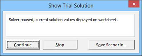
Figure 17.7 When the Show Iteration Results check box is selected, Solver displays the Show Trial Solution dialog box so that you can view each intermediate solution.
![]() Ignore Integer Constraints—Integer programming (in which you have integer constraints) can take a long time because of the complexity involved in finding solutions that satisfy exact integer constraints. If you find your models taking an abnormally long time to solve, select this check box. (Alternatively, increase the value in the Integer Optimality box, discussed next, to get an approximate solution.)
Ignore Integer Constraints—Integer programming (in which you have integer constraints) can take a long time because of the complexity involved in finding solutions that satisfy exact integer constraints. If you find your models taking an abnormally long time to solve, select this check box. (Alternatively, increase the value in the Integer Optimality box, discussed next, to get an approximate solution.)
![]() Integer Optimality—If you have integer constraints, this box determines what percentage of the integer Solver has to be within before declaring the constraint satisfied. For example, if the integer tolerance is set to 5 (that is, 0.05%), Solver will declare a cell with the value 99.95 to be close enough to 100 to declare it an integer.
Integer Optimality—If you have integer constraints, this box determines what percentage of the integer Solver has to be within before declaring the constraint satisfied. For example, if the integer tolerance is set to 5 (that is, 0.05%), Solver will declare a cell with the value 99.95 to be close enough to 100 to declare it an integer.
![]() Max Time—The amount of time Solver takes is a function of the size and complexity of the model, the number of variable cells and constraint cells, and the other Solver options you’ve chosen. If you find that Solver runs out of time before finding a solution, increase the number in this text box.
Max Time—The amount of time Solver takes is a function of the size and complexity of the model, the number of variable cells and constraint cells, and the other Solver options you’ve chosen. If you find that Solver runs out of time before finding a solution, increase the number in this text box.
![]() Iterations—This box controls the number of iterations Solver tries before giving up on a problem. Increasing this number gives Solver more of a chance to solve the problem, but it takes correspondingly longer.
Iterations—This box controls the number of iterations Solver tries before giving up on a problem. Increasing this number gives Solver more of a chance to solve the problem, but it takes correspondingly longer.
![]() Max Subproblems—If you use the Evolutionary engine or if you deselect the Ignore Integer Constraints check box, the value in the Max Subproblems box tells Solver the maximum number of subproblems it can investigate before it asks if you want to continue. A subproblem is an intermediate step that Solver uses to get closer to the final solution.
Max Subproblems—If you use the Evolutionary engine or if you deselect the Ignore Integer Constraints check box, the value in the Max Subproblems box tells Solver the maximum number of subproblems it can investigate before it asks if you want to continue. A subproblem is an intermediate step that Solver uses to get closer to the final solution.
![]() Max Feasible Solutions—If you use the Evolutionary engine or if you deselect the Ignore Integer Constraints check box, the value in the Max Feasible Solutions box tells Solver the maximum number of feasible solutions that it can generate before it asks if you want to continue. Afeasible solution is any solution (even a nonoptimal one) that satisfies all the constraints.
Max Feasible Solutions—If you use the Evolutionary engine or if you deselect the Ignore Integer Constraints check box, the value in the Max Feasible Solutions box tells Solver the maximum number of feasible solutions that it can generate before it asks if you want to continue. Afeasible solution is any solution (even a nonoptimal one) that satisfies all the constraints.
If you want to use the GRG Nonlinear engine, consider the following options in the GRG Nonlinear tab:
![]() Convergence—This number determines when Solver decides that it has reached (converged on) a solution. If the objective cell value changes by less than the Convergence value for five straight iterations, then Solver decides that a solution has been found, and it stops iterating. Enter a number between 0 and 1, keeping in mind that the smaller the number, the more accurate the solution will be but also the longer Solver will take to find a solution.
Convergence—This number determines when Solver decides that it has reached (converged on) a solution. If the objective cell value changes by less than the Convergence value for five straight iterations, then Solver decides that a solution has been found, and it stops iterating. Enter a number between 0 and 1, keeping in mind that the smaller the number, the more accurate the solution will be but also the longer Solver will take to find a solution.
![]() Derivatives—Some models require Solver to calculate partial derivatives. The two Derivatives options specify the method Solver uses to do this. Forward differencing is the default method. The Central differencing method takes longer than forward differencing, but you might want to try it when Solver reports that it can’t improve a solution. (See the section “Making Sense of Solver’s Messages,” later in this chapter.)
Derivatives—Some models require Solver to calculate partial derivatives. The two Derivatives options specify the method Solver uses to do this. Forward differencing is the default method. The Central differencing method takes longer than forward differencing, but you might want to try it when Solver reports that it can’t improve a solution. (See the section “Making Sense of Solver’s Messages,” later in this chapter.)
![]() Use Multistart—Select this check box to run the GRG Nonlinear engine using its Multistart feature. This means that Solver automatically runs the GRG Nonlinear engine from a number of different starting points, which Solver selects at random (although see the Require Bounds on Variables item, later in the list, for more information on this). Solver then gathers the points that produced locally optimal solutions and compares them to come up with a globally optimal solution. Use Multistart if the GRG Nonlinear engine is having trouble finding a solution to your model.
Use Multistart—Select this check box to run the GRG Nonlinear engine using its Multistart feature. This means that Solver automatically runs the GRG Nonlinear engine from a number of different starting points, which Solver selects at random (although see the Require Bounds on Variables item, later in the list, for more information on this). Solver then gathers the points that produced locally optimal solutions and compares them to come up with a globally optimal solution. Use Multistart if the GRG Nonlinear engine is having trouble finding a solution to your model.
![]() Population Size—If you select the Use Multistart check box, use this text box to set the number of starting points that Solver uses. If Solver has trouble finding a globally optimal solution, try increasing the population size; if Solver takes a long time to find a globally optimal solution, try reducing the population size.
Population Size—If you select the Use Multistart check box, use this text box to set the number of starting points that Solver uses. If Solver has trouble finding a globally optimal solution, try increasing the population size; if Solver takes a long time to find a globally optimal solution, try reducing the population size.
![]() Random Seed—If you select the Use Multistart check box, Solver generates random starting points for the GRG Nonlinear engine, and the random number generator is seeded with the current system clock value. This is almost always the best way to go. However, if you want to ensure that the GRG Nonlinear engine always uses the same starting points for consecutive runs, enter an integer (nonzero) value in the Random Seed text box.
Random Seed—If you select the Use Multistart check box, Solver generates random starting points for the GRG Nonlinear engine, and the random number generator is seeded with the current system clock value. This is almost always the best way to go. However, if you want to ensure that the GRG Nonlinear engine always uses the same starting points for consecutive runs, enter an integer (nonzero) value in the Random Seed text box.
![]() Require Bounds on Variables—Leave this check box selected to improve the likelihood that the GRG Nonlinear engine finds a solution when you use the Multistart method. This means that you must add constraints that specify both a lower bound and an upper bound for each cell in the By Changing Variable Cells range box. When Solver generates the random starting points for the GRG Nonlinear engine, it generates values that are within these lower and upper bounds, so it’s more likely to find a solution (assuming that you enter realistic bounds for the variable cells). It’s possible to use the GRG Nonlinear engine if you deselect the Require Bounds on Variables check box, but it means that Solver must select its random starting points from, essentially, an infinite supply of values, so it’s less likely to find a globally optimal solution.
Require Bounds on Variables—Leave this check box selected to improve the likelihood that the GRG Nonlinear engine finds a solution when you use the Multistart method. This means that you must add constraints that specify both a lower bound and an upper bound for each cell in the By Changing Variable Cells range box. When Solver generates the random starting points for the GRG Nonlinear engine, it generates values that are within these lower and upper bounds, so it’s more likely to find a solution (assuming that you enter realistic bounds for the variable cells). It’s possible to use the GRG Nonlinear engine if you deselect the Require Bounds on Variables check box, but it means that Solver must select its random starting points from, essentially, an infinite supply of values, so it’s less likely to find a globally optimal solution.
If you want to use the Evolutionary engine, you can configure the engine using the options in the Evolutionary tab. The Convergence, Population Size, Random Seed, and Require Bounds on Variables options are the same as those in the GRG Nonlinear tab, discussed earlier. The Evolutionary tab has the following unique options:
![]() Mutation Rate—The Evolutionary engine operates by randomly trying out certain values, usually within upper and lower bounds of the variable cells (assuming that you leave the Require Bounds on Variables check box selected), and if a trial solution is found to be “fit,” that result becomes part of the solution population. It then mutates members of this population to see if it can find better solutions. The Mutation Rate value is the probability that a member of the solution population will be mutated. If you’re having trouble getting good results from the Evolutionary engine, try increasing the mutation rate.
Mutation Rate—The Evolutionary engine operates by randomly trying out certain values, usually within upper and lower bounds of the variable cells (assuming that you leave the Require Bounds on Variables check box selected), and if a trial solution is found to be “fit,” that result becomes part of the solution population. It then mutates members of this population to see if it can find better solutions. The Mutation Rate value is the probability that a member of the solution population will be mutated. If you’re having trouble getting good results from the Evolutionary engine, try increasing the mutation rate.
![]() Maximum Time Without Improvement—This is the maximum number of seconds the Evolutionary engine will take without finding a better solution before it asks if you want to stop the iteration. If you find that the Evolutionary engine runs out of time before finding a solution, increase the number in this text box.
Maximum Time Without Improvement—This is the maximum number of seconds the Evolutionary engine will take without finding a better solution before it asks if you want to stop the iteration. If you find that the Evolutionary engine runs out of time before finding a solution, increase the number in this text box.
Working with Solver Models
Excel attaches your most recent Solver parameters to the worksheet when you save it. If you want to save different sets of parameters, you can do so by following these steps:
1. Select Data, Solver to display the Solver Parameters dialog box.
2. Enter the parameters you want to save.
3. Click Options to display the Options dialog box.
4. Enter the options you want to save and then click OK to return to the Solver Parameters dialog box.
5. Click Load/Save. Solver displays the Load/Save Model dialog box to prompt you to enter a range in which to store the model.
6. Enter the range in the range box. Note that you don’t need to specify the entire area—just the first cell. Keep in mind that Solver displays the data in a column, so pick a cell with enough empty space below it to hold all the data. You’ll need one cell for the objective cell reference, one for the variable cells, one for each constraint, and one to hold the array of Solver options.
7. Click Save. Solver gathers the data, enters it into your selected range, and then returns you to the Solver Parameters dialog box.
Figure 17.8 shows an example of a saved model (the range F4:F8). I’ve changed the worksheet view to show formulas, and I’ve added some explanatory text so you can see exactly how Solver saves the model. Notice that the formula for the objective cell (F4) includes both the target (B14) and the target value (=0).
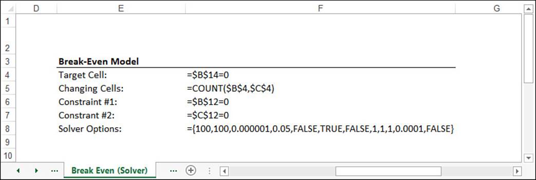
Figure 17.8 A saved Solver model with formulas turned on so you can see what Solver saves to the sheet.
Note
To toggle formulas on and off in Excel, select Formulas, Show Formulas or press Ctrl+` (backquote).
To use your saved settings, follow these steps:
1. Select Data, Solver to display the Solver Parameters dialog box.
2. Click Load/Save. Solver displays the Load/Save Model dialog box.
3. Select the entire range that contains the saved model.
4. Click Load. Excel asks if you want to replace the current model or merge the saved model with the current model.
5. Click Replace to use the saved model cells or click Merge to add the saved model to the current Solver model. Excel returns you to the Solver Parameters dialog box.
Making Sense of Solver’s Messages
When Solver finishes its calculations, it displays the Solver Results dialog box and a message that tells you what happened. Some of these messages are straightforward, but others are more than a little cryptic. This section looks at the most common messages and gives their translations.
If Solver finds a solution successfully, you see one of the following messages:
![]() Solver found a solution. All constraints and optimality conditions are satisfied—This is the message you hope to see. It means that the value you wanted for the objective cell has been found, and Solver was able to find the solution while meeting your constraints within the precision and integer tolerance levels you set.
Solver found a solution. All constraints and optimality conditions are satisfied—This is the message you hope to see. It means that the value you wanted for the objective cell has been found, and Solver was able to find the solution while meeting your constraints within the precision and integer tolerance levels you set.
![]() Solver has converged to the current solution. All constraints are satisfied—Solver normally assumes that it has a solution if the value of the objective cell formula remains virtually unchanged during a few iterations. This is called converging to a solution. Such is the case with this message, but it doesn’t necessarily mean that Solver has found a solution. The iterative process might just be taking a long time, or the initial values in the variable cells might have been set too far from the solution. You should try rerunning Solver with different values. You also can try using a higher precision setting (that is, entering a smaller number in the Constraint Precision text box).
Solver has converged to the current solution. All constraints are satisfied—Solver normally assumes that it has a solution if the value of the objective cell formula remains virtually unchanged during a few iterations. This is called converging to a solution. Such is the case with this message, but it doesn’t necessarily mean that Solver has found a solution. The iterative process might just be taking a long time, or the initial values in the variable cells might have been set too far from the solution. You should try rerunning Solver with different values. You also can try using a higher precision setting (that is, entering a smaller number in the Constraint Precision text box).
![]() Solver cannot improve the current solution. All constraints are satisfied—This message tells you that Solver has found a solution, but it might not be the optimal one. Try setting the precision to a smaller number or, if you’re using the GRG Nonlinear engine, try using the central differencing method for partial derivatives.
Solver cannot improve the current solution. All constraints are satisfied—This message tells you that Solver has found a solution, but it might not be the optimal one. Try setting the precision to a smaller number or, if you’re using the GRG Nonlinear engine, try using the central differencing method for partial derivatives.
If Solver doesn’t find a solution, you see one of the following messages telling you why:
![]() The Set Cell values do not converge—This means that the value of the objective cell formula has no finite limit. For example, if you’re trying to maximize profit based on product price and unit costs, Solver won’t find a solution; the reason is that continually higher prices and lower costs lead to higher profit. You need to add (or change) constraints in your model, such as setting a maximum price or minimum cost level (for example, the amount of fixed costs).
The Set Cell values do not converge—This means that the value of the objective cell formula has no finite limit. For example, if you’re trying to maximize profit based on product price and unit costs, Solver won’t find a solution; the reason is that continually higher prices and lower costs lead to higher profit. You need to add (or change) constraints in your model, such as setting a maximum price or minimum cost level (for example, the amount of fixed costs).
![]() Solver could not find a feasible solution—Solver couldn’t find a solution that satisfied all your constraints. Check your constraints to make sure they’re realistic and consistent.
Solver could not find a feasible solution—Solver couldn’t find a solution that satisfied all your constraints. Check your constraints to make sure they’re realistic and consistent.
![]() Stop chosen when the maximum x limit was reached—This message appears when Solver bumps up against either the maximum time limit or the maximum iteration limit. If it appears that Solver is heading toward a solution, click Keep Solver Solution and try again.
Stop chosen when the maximum x limit was reached—This message appears when Solver bumps up against either the maximum time limit or the maximum iteration limit. If it appears that Solver is heading toward a solution, click Keep Solver Solution and try again.
![]() The conditions for Assume Linear Model are not satisfied—Solver based its iterative process on a linear model, but when the results are put into the worksheet, they don’t conform to the linear model. You need to select the GRG Nonlinear engine and try again.
The conditions for Assume Linear Model are not satisfied—Solver based its iterative process on a linear model, but when the results are put into the worksheet, they don’t conform to the linear model. You need to select the GRG Nonlinear engine and try again.
Case Study: Solving the Transportation Problem
The best way to learn how to use a complex tool such as Solver is to get your hands dirty with some examples. Excel thoughtfully comes with several sample worksheets that use simplified models to demonstrate the various problems Solver can handle. This case study looks at one of these worksheets in detail.
The transportation problem is the classic model for solving linear programming problems. The basic goal is to minimize the costs of shipping goods from several production plants to various warehouses scattered around the country. Your constraints are as follows:
![]() The amount shipped to each warehouse must meet the warehouse’s demand for goods.
The amount shipped to each warehouse must meet the warehouse’s demand for goods.
![]() The amount shipped from each plant must be greater than or equal to 0.
The amount shipped from each plant must be greater than or equal to 0.
![]() The amount shipped from each plant can’t exceed the plant’s supply of goods.
The amount shipped from each plant can’t exceed the plant’s supply of goods.
Figure 17.9 shows the model for solving the transportation problem.
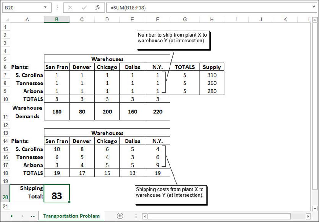
Figure 17.9 A worksheet for solving the transportation problem.
The top table (A6:F10) lists the three plants (A7:A9) and the five warehouses (B6:F6). This table holds the number of units shipped from each plant to each warehouse. In the Solver model, these are the variable cells. The total shipped to each warehouse (B10:F10) must match the warehouse demands (B11:F11) to satisfy constraint number 1. The amount shipped from each plant (B7:F9) must be greater than or equal to 0 to satisfy constraint number 2. The total shipped from each plant (G7:G9) must be less than or equal to the available supply for each plant (H7:H9) to satisfy constraint number 3.
Note
When you need to use a range of values in a constraint, you don’t need to set up a separate constraint for each cell. Instead, you can compare entire ranges. For example, the constraint that the total shipped from each plant must be less than or equal to the plant supply can be entered as follows:
G7:G9 <= H7:H9
The bottom table (A14:F18) holds the corresponding shipping costs from each plant to each warehouse. The total shipping cost (cell B20) is the objective cell you want to minimize.
Figure 17.10 shows the final Solver Parameters dialog box that you’ll use to solve this problem. (Note also that I selected the Simplex LP engine in the Select a Solver Method list.) Figure 17.11 shows the solution that Solver found.
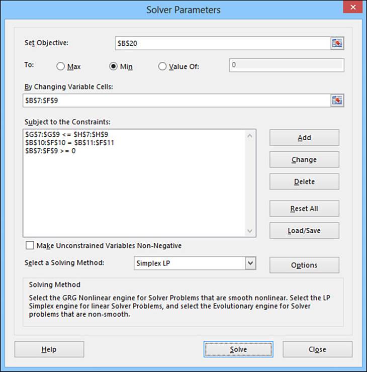
Figure 17.10 The Solver Parameters dialog box filled in for the transportation problem.
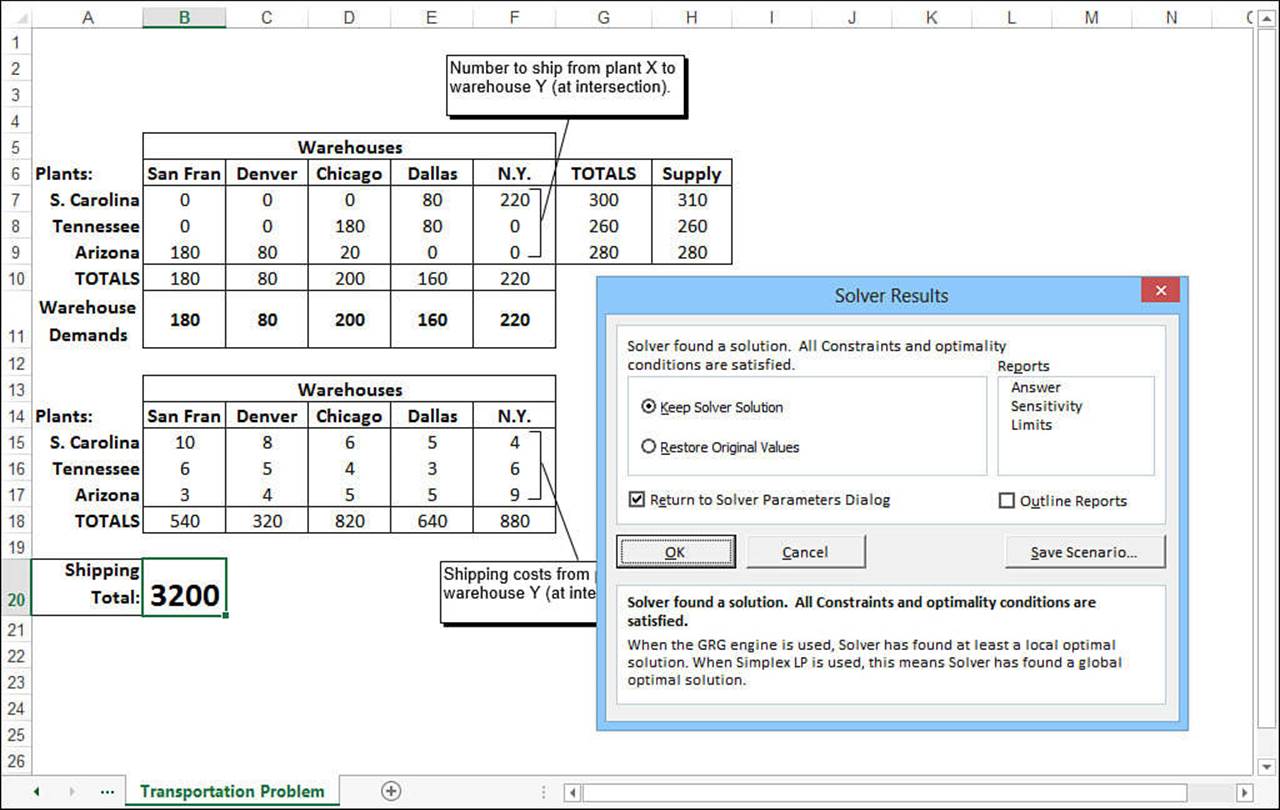
Figure 17.11 The optimal solution for the transportation problem.
Displaying Solver’s Reports
When Solver finds a solution, the Solver dialog box gives you the option of generating three reports: the Answer report, Sensitivity report, and Limits report. Click the reports you want to see in the Reports list box and then click OK. Excel displays each report on its own worksheet.
Tip
If you’ve named the cells in your model, Solver uses these names to make its reports easier to read. If you haven’t already done so, you should define names for the objective cell, variable cells, and constraint cells before creating a report.
The Answer Report
The Answer report displays information about the model’s objective cell, variable cells, and constraints. For the objective cell and variable cells, Solver shows the original and final values. For example, Figure 17.12 shows this portion of the answer report for the transportation problem solution.
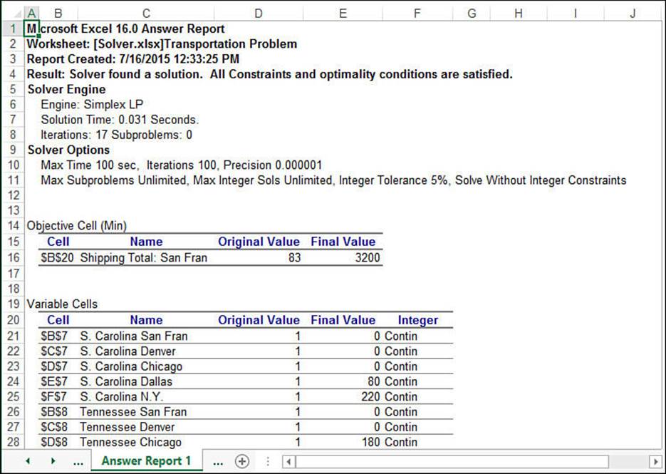
Figure 17.12 The Objective Cell and Variable Cells sections of Solver’s Answer report.
For the constraints, the report shows the address and name for each cell, the final value, the formulas, and two values called the status and the slack. Figure 17.13 shows an example from the transportation problem. The status can be one of three values:
![]() Binding—The final value in the constraint cell equals the constraint value (or the constraint boundary, if the constraint is an inequality).
Binding—The final value in the constraint cell equals the constraint value (or the constraint boundary, if the constraint is an inequality).
![]() Not Binding—The constraint cell value satisfied the constraint, but it doesn’t equal the constraint boundary.
Not Binding—The constraint cell value satisfied the constraint, but it doesn’t equal the constraint boundary.
![]() Not Satisfied—The constraint was not satisfied.
Not Satisfied—The constraint was not satisfied.
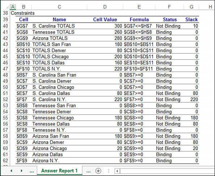
Figure 17.13 The Constraints section of Solver’s Answer report.
The slack is the difference between the final constraint cell value and the value of the original constraint (or its boundary). In the optimal solution for the transportation problem, for example, the total shipped from the South Carolina plant is 300, but the constraint on this total was 310 (the total supply). Therefore, the slack value is 10 (or close enough to it). If the status is binding, the slack value is always 0.
The Sensitivity Report
The Sensitivity report attempts to show how sensitive a solution is to changes in the model’s formulas. The layout of the Sensitivity report depends on the type of model you’re using. For a linear model (that is, a model in which you selected the Simplex LP engine), you see a report similar to the one shown in Figure 17.14.
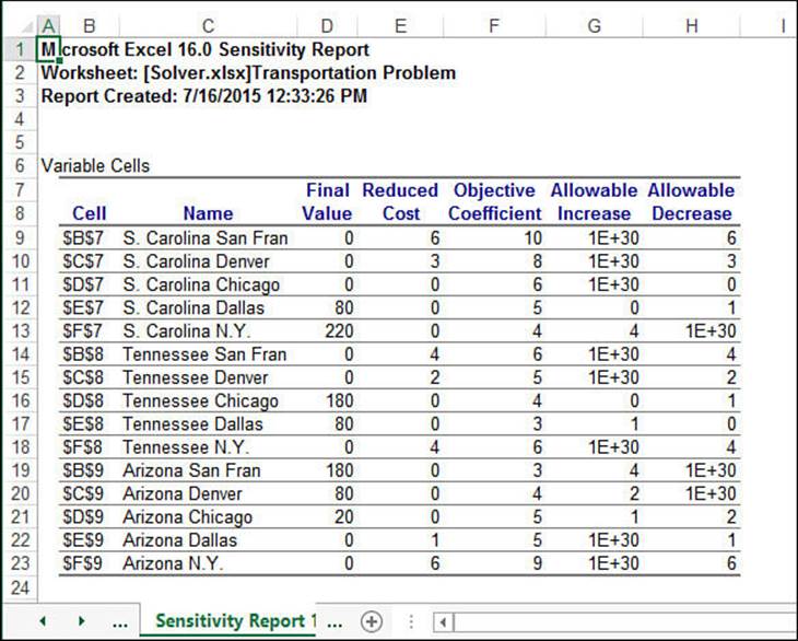
Figure 17.14 The Variable Cells section of Solver’s Sensitivity report.
This report is divided into two sections. The top section, called Variable Cells, shows for each cell the address and name of the cell, its final value, and the following measures:
![]() Reduced Cost—The corresponding increase in the objective cell, given a one-unit increase in the variable cell
Reduced Cost—The corresponding increase in the objective cell, given a one-unit increase in the variable cell
![]() Objective Coefficient—The relative relationship between the variable cell and the objective cell
Objective Coefficient—The relative relationship between the variable cell and the objective cell
![]() Allowable Increase—The change in the objective coefficient before there would be an increase in the optimal value of the variable cell
Allowable Increase—The change in the objective coefficient before there would be an increase in the optimal value of the variable cell
![]() Allowable Decrease—The change in the objective coefficient before there would be a decrease in the optimal value of the variable cell
Allowable Decrease—The change in the objective coefficient before there would be a decrease in the optimal value of the variable cell
The bottom section of the Sensitivity report, called Constraints (see Figure 17.15), shows for each constraint cell the address and name of the cell, its final value, and the following values:
![]() Shadow Price—The corresponding increase in the objective cell, given a one-unit increase in the constraint value
Shadow Price—The corresponding increase in the objective cell, given a one-unit increase in the constraint value
![]() Constraint R.H. Side—The constraint value that you specified (that is, the right-hand side of the constraint equation)
Constraint R.H. Side—The constraint value that you specified (that is, the right-hand side of the constraint equation)
![]() Allowable Increase—The change in the constraint value before there would be an increase in the optimal value of the variable cell
Allowable Increase—The change in the constraint value before there would be an increase in the optimal value of the variable cell
![]() Allowable Decrease—The change in the constraint value before there would be a decrease in the optimal value of the variable cell.
Allowable Decrease—The change in the constraint value before there would be a decrease in the optimal value of the variable cell.
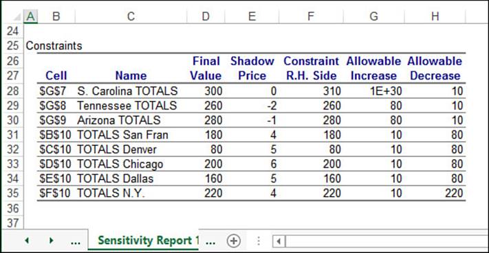
Figure 17.15 The Constraints section of Solver’s Sensitivity report.
The Sensitivity report for a nonlinear model shows the variable cells and the constraint cells. For each cell, the report displays the address, name, and final value. The Variable Cells section also shows the Reduced Gradient value, which measures the corresponding increase in the objective cell, given a one-unit increase in the variable cell (similar to the Reduced Cost measure for a linear model). The Constraints section also shows the Lagrange Multiplier value, which measures the corresponding increase in the objective cell, given a one-unit increase in the constraint value (similar to the Shadow Price in the linear report).
The Limits Report
The Limits report, shown in Figure 17.16, displays the objective cell and its value, as well as the variable cells and their addresses, names, values, and the following measures:
![]() Lower Limit—The minimum value that the variable cell can assume while keeping the other variable cells fixed and still satisfying the constraints
Lower Limit—The minimum value that the variable cell can assume while keeping the other variable cells fixed and still satisfying the constraints
![]() Upper Limit—The maximum value that the variable cell can assume while keeping the other variable cells fixed and still satisfying the constraints
Upper Limit—The maximum value that the variable cell can assume while keeping the other variable cells fixed and still satisfying the constraints
![]() Objective Result—The objective cell’s value when the variable cell is at the lower limit or upper limit
Objective Result—The objective cell’s value when the variable cell is at the lower limit or upper limit
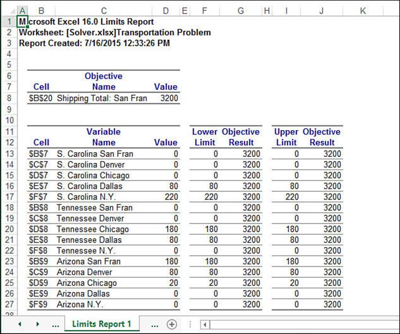
Figure 17.16 Solver’s Limits report.
From Here
![]() To learn about using iteration to solve problems, see “Using Iteration and Circular References,” p. 93.
To learn about using iteration to solve problems, see “Using Iteration and Circular References,” p. 93.
![]() For simple models, the Goal Seek tool might be all you need. See “Working with Goal Seek,” p. 355.
For simple models, the Goal Seek tool might be all you need. See “Working with Goal Seek,” p. 355.
![]() To learn about scenarios, see “Working with Scenarios,” p. 362.
To learn about scenarios, see “Working with Scenarios,” p. 362.
All materials on the site are licensed Creative Commons Attribution-Sharealike 3.0 Unported CC BY-SA 3.0 & GNU Free Documentation License (GFDL)
If you are the copyright holder of any material contained on our site and intend to remove it, please contact our site administrator for approval.
© 2016-2026 All site design rights belong to S.Y.A.