Excel® 2016 Formulas and Functions (2016)
Part IV: Building Financial Formulas
18. Building Loan Formulas
In This Chapter
Understanding the Time Value of Money
Calculating a Loan Payment
Building a Loan Amortization Schedule
Calculating the Term of a Loan
Calculating the Interest Rate Required for a Loan
Calculating How Much You Can Borrow
Excel is loaded with financial features that give you powerful tools for building worksheets that manage both business and personal finances. You can use these functions to calculate such things as the monthly payment on a loan, the future value of an annuity, the internal rate of return of an investment, or the yearly depreciation of an asset. The final three chapters of this book cover these and many other uses for Excel’s financial formulas.
This chapter covers formulas and functions related to loans and mortgages. You’ll learn about the time value of money; how to calculate loan payments, loan periods, the principal and interest components of a payment, and the interest rate; and how to build an amortization schedule.
Understanding the Time Value of Money
The time value of money means that a dollar in hand now is worth more than a dollar promised at some future date. This seemingly simple idea underlies not only the concepts and techniques you learn in this chapter but also the investment formulas in Chapter 19, “Building Investment Formulas,” and the discount formulas in Chapter 20, “Building Discount Formulas.” A dollar now is worth more than a dollar promised in the future for two reasons:
![]() You can invest a dollar now. If you earn a positive return, the sum of the dollar and interest earned will be worth more than the future dollar.
You can invest a dollar now. If you earn a positive return, the sum of the dollar and interest earned will be worth more than the future dollar.
![]() You might never see the future dollar. Due to bankruptcy, cash-flow problems, or any number of other reasons, there’s a risk that the company or person promising you the future dollar might not be able to deliver it.
You might never see the future dollar. Due to bankruptcy, cash-flow problems, or any number of other reasons, there’s a risk that the company or person promising you the future dollar might not be able to deliver it.
These two factors—interest and risk—are at the heart of most financial formulas and models. More realistically, these factors really mean that you’re mostly comparing the benefits of investing a dollar now versus getting a dollar in the future plus some risk premium—an amount that compensates for the risk you’re taking in waiting for the dollar to be delivered.
You compare these by looking at the present value (the amount something is worth now) and the future value (the amount something is worth in the future). They’re related as follows:
A. Future value = Present value + Interest
B. Present value = Future value − discount
Much financial analysis boils down to comparing these formulas. If the present value in A is greater than the present value in B, A is the better investment; conversely, if the future value in B is better than the future value in A, B is the better investment.
Most of the formulas you’ll work with over the next three chapters involve these three factors—the present value, the future value, and the interest rate (or the discount rate)—plus two related factors: the periods, which are the number of payments or deposits over the term of the loan or investment, and the payment, which is the amount of money paid out or invested in each period.
When building your financial formulas, you need to ask yourself the following questions:
![]() Who or what is the subject of the formula? On a mortgage analysis, for example, are you performing the analysis on behalf of yourself or the bank?
Who or what is the subject of the formula? On a mortgage analysis, for example, are you performing the analysis on behalf of yourself or the bank?
![]() Which way is the money flowing with respect to the subject? For the present value, future value, and payment, enter money that the subject receives as a positive quantity and enter money that the subject pays out as a negative quantity. For example, if you’re the subject of a mortgage analysis, the loan principal (the present value) is a positive number because it’s money that you receive from the bank; the payment and the remaining principal (the future value) are negative because they’re amounts that you pay to the bank.
Which way is the money flowing with respect to the subject? For the present value, future value, and payment, enter money that the subject receives as a positive quantity and enter money that the subject pays out as a negative quantity. For example, if you’re the subject of a mortgage analysis, the loan principal (the present value) is a positive number because it’s money that you receive from the bank; the payment and the remaining principal (the future value) are negative because they’re amounts that you pay to the bank.
![]() What is the time unit? The underlying unit of both the interest rate and the period must be the same. For example, if you’re working with the annual interest rate, you must express the period in years. Similarly, if you’re working with monthly periods, you must use a monthly interest rate.
What is the time unit? The underlying unit of both the interest rate and the period must be the same. For example, if you’re working with the annual interest rate, you must express the period in years. Similarly, if you’re working with monthly periods, you must use a monthly interest rate.
![]() When are the payments made? Excel differentiates between payments made at the end of each period and those made at the beginning.
When are the payments made? Excel differentiates between payments made at the end of each period and those made at the beginning.
Calculating a Loan Payment
When negotiating a loan to purchase equipment or a mortgage for your house, the first concern that comes up is almost always the size of the payment you’ll need to make each period. This is just basic cash-flow management because the monthly (or whatever) payment must fit within your budget.
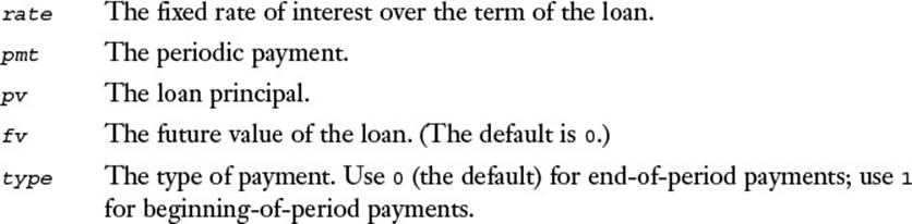
To return the periodic payment for a loan, use the PMT() function:
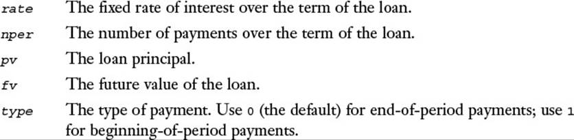
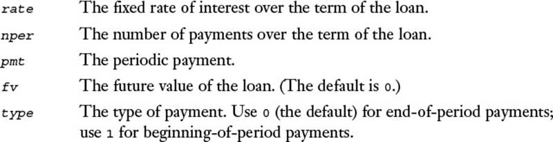
PMT(rate, nper, pv[, fv][, type])
For example, the following formula returns the monthly payment of a $10,000 loan with an annual interest rate of 6% (0.5% per month) over five years (60 months):
=PMT(0.005, 60, 10000)
Loan Payment Analysis
Financial formulas rarely use hard-coded function arguments. Instead, you almost always are better off placing the argument values in separate cells and then referring to those cells in the formula. This enables you to do a rudimentary form of loan analysis by plugging in different argument values and seeing the effects they have on the formula result.
Figure 18.1 shows an example of a worksheet set up to perform such an analysis. The PMT() formula is in cell B7, and the function arguments are stored in B4 (rate), B5 (nper), and B6 (pv).
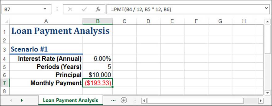
Figure 18.1 To perform a simple loan analysis, place the PMT() function arguments in separate cells and then change those cell values to see the effect on the formula.
Note
You can download this chapter’s sample workbook at www.mcfedries.com/books/book.php?title=excel-2016-formulas-and-functions.
Note two things about the formula and result in cell B7:
![]() The interest rate is an annual value, and the periods are expressed in years, so to get a monthly payment, you must convert these values to their monthly equivalents. This means that the interest rate is divided by 12 and the number of periods is multiplied by 12:
The interest rate is an annual value, and the periods are expressed in years, so to get a monthly payment, you must convert these values to their monthly equivalents. This means that the interest rate is divided by 12 and the number of periods is multiplied by 12:
=PMT(B4 / 12, B5 * 12, B6)
![]() The PMT() function returns a negative value, which is correct because this worksheet is set up from the point of view of the person receiving the loan, and the payment is money that flows away from that person.
The PMT() function returns a negative value, which is correct because this worksheet is set up from the point of view of the person receiving the loan, and the payment is money that flows away from that person.
Working with a Balloon Loan
Many loans are set up so that the payments take care of only a portion of the principal, with the remainder due as an end-of-loan balloon payment. This balloon payment is the future value of the loan, so you need to factor it into the PMT() function as the fv argument.
You might think that the pv argument should be the partial principal—that is, the original loan principal minus the balloon amount. This seems right because the loan term is designed to pay off the partial principal. That’s not the case, however. In a balloon loan, you also pay interest on the balloon part of the principal. That is, each payment in a balloon loan has three components:
![]() A paydown of the partial principal
A paydown of the partial principal
![]() Interest on the partial principal
Interest on the partial principal
![]() Interest on the balloon portion of the principal
Interest on the balloon portion of the principal
Therefore, the PMT() function’s pv argument must be the entire principal, with the balloon portion as the (negative) fv argument.
For example, suppose that the loan from the previous section has a $3,000 balloon payment. Figure 18.2 shows a new worksheet that adds the balloon payment to the model and then calculates the payment using the following revised formula:
=PMT(B2 / 12, B3 * 12, B4, -B5)
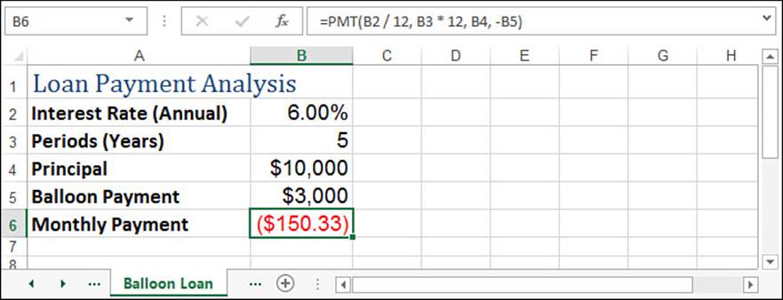
Figure 18.2 To allow for an end-of-loan balloon payment, add the fv argument to the PMT() function.
Note that the balloon payment is entered into the worksheet as a positive value (because it represents, in this model, money going out), so the negation operation is used in the formula (-B5) to convert it to a negative value.
Calculating Interest Costs, Part 1
When you know the payment, you can calculate the total interest costs of a loan by first figuring the total of all the payments and then subtracting the principal. The remainder is the total interest paid over the life of the loan.
Figure 18.3 shows a worksheet that performs this calculation. In column B, cell B7 contains the total amount paid (the monthly payment multiplied by the number of months), and cell B8 takes the difference. Column C performs the same calculations on the loan with a balloon payment. As you can see, in the balloon payment scenario, the payment total is about $2,600 smaller, but the total interest is about $400 higher.
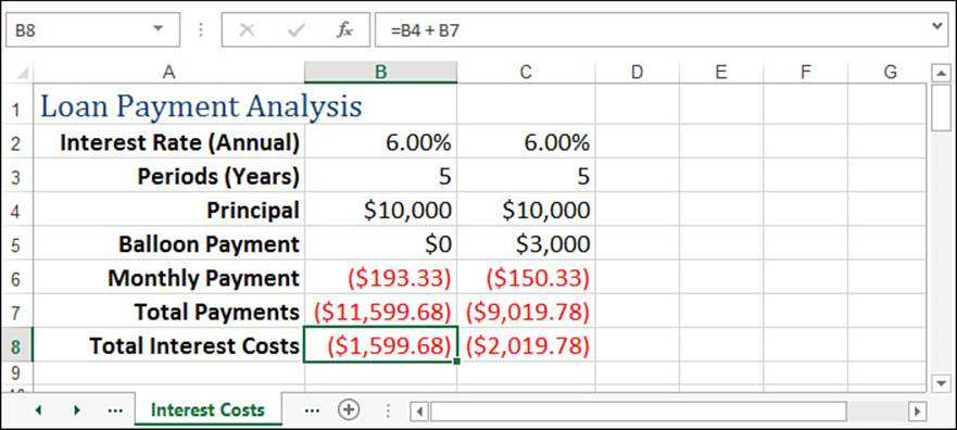
Figure 18.3 To calculate total interest paid out over the life of a loan, multiply the periodic payment by the number of periods and then subtract the principal paid.
Calculating the Principal and Interest
Any loan payment has two components: principal repayment and interest charges. Interest charges are almost always front loaded, which means that the interest component is highest at the beginning of the loan and gradually decreases with each payment. This means, conversely, that the principal component increases gradually with each payment.
To calculate the principal and interest components of a loan payment, use the PPMT() and IPMT() functions, respectively:
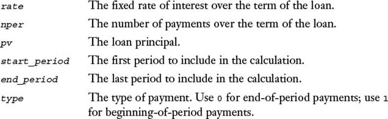
PPMT(rate, per, nper, pv[, fv][, type])
IPMT(rate, per, nper, pv[, fv][, type])
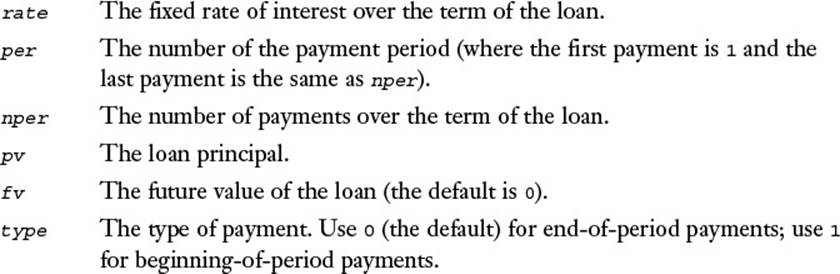
Figure 18.4 shows a worksheet that applies these functions to the loan. The table shows the principal (column F) and interest (column G) components of the loan for the first 10 periods and for the final period. Note that with each period, the principal portion increases and the interest portion decreases. However, the total remains the same (as confirmed by the Total column), which is as it should be because the payment remains constant through the life of the loan.
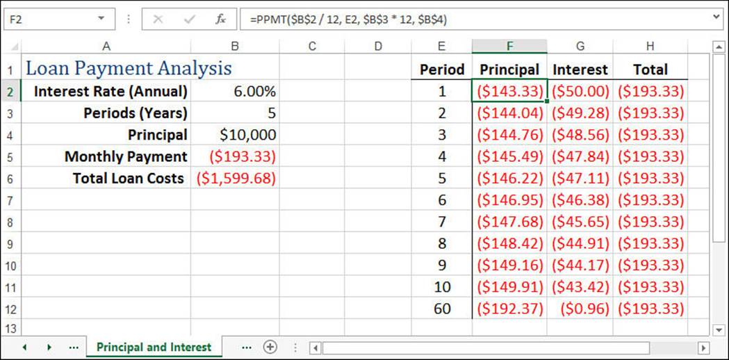
Figure 18.4 This worksheet uses the PPMT() and IPMT() functions to break out the principal and interest components of a loan payment.
Calculating Interest Costs, Part 2
Another way to calculate the total interest paid on a loan is to sum the various IPMT() values over the life of the loan. You can do this by using an array formula that generates the values of the IPMT() function’s per argument. Here’s the general formula:
{=IPMT(rate, ROW(INDIRECT("A1:A" & nper)), nper, pv[, fv][, type])}
The array of per values is generated by the following expression:
ROW(INDIRECT("A1:A" & nper))
The INDIRECT() function converts a string range reference into an actual range reference, and then the ROW() function returns the row numbers from that range. By starting the range at A1, this expression generates integer values from 1 to nper, which covers the life of the loan.
For example, here’s a formula that calculates the total interest cost of the loan model shown in Figure 18.4:
{=SUM(IPMT(B2 / 12, ROW(INDIRECT("A1:A" & B3 * 12)), B3 * 12, B4))}
Caution
The array formula doesn’t work if the loan includes a balloon payment.
Calculating Cumulative Principal and Interest
Knowing how much principal and interest you pay each period is useful, but it’s usually handier to know how much principal or interest you’ve paid in total up to a given period. For example, if you sign up for a mortgage with a five-year term, how much principal will you have paid off by the end of the term? Similarly, a business might need to know the total interest payments a loan requires in the first year so that it can factor the result into its expense budgeting.
You could solve these kinds of problems by building a model that uses the PPMT() and IPMT() functions over the time frame you’re dealing with and then summing the results. However, Excel has two functions that offer a more direct route:
CUMPRINC(rate, nper, pv, start_period, end_period, type)
CUMIPMT(rate, nper, pv, start_period, end_period, type)
Caution
In both CUMPRINC() and CUMIPMT(), all of the arguments are required. If you omit the type argument (which is optional in most other financial functions), Excel returns the #N/A error.
The main difference between CUMPRINC() and CUMIPMT() and PPMT() and IPMT() is the start_period and end_period arguments. For example, to find the cumulative principal or interest in the first year of a loan, you set start_period to 1 and end_period to 12; for the second year, you set start_period to 13 and end_period to 24. Here are a couple of formulas that calculate these values for any year, assuming that the year value (1, 2, and so on) is in cell D2:
start_period: (D2 - 1) * 12 + 1
end_period: D2 * 12
Figure 18.5 shows a worksheet that returns the cumulative principal and interest paid in each year of a loan, as well as the total principal and interest for all five years.
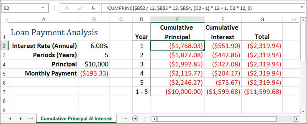
Figure 18.5 This worksheet uses the CUMPRINC() and CUMIPMT() functions to return the cumulative principal and interest for each year of a loan.
Note
Note that the CUMIPMT() function gives you an easier way to calculate the total interest costs for a loan. Just set start_period to 1 and end_period to the number of periods (the value of nper).
Caution
Although the CUMPRINC() function works as advertised if the loan includes a balloon payment, the CUMIPMT() function does not.
Building a Loan Amortization Schedule
A loan amortization schedule is a table that shows a sequence of calculations over the life of a loan. For each period, the schedule shows figures such as the payment, the principal and interest components of the payment, the cumulative principal and interest, and the remaining principal. The next few sections take you through various amortization schedules designed for different scenarios.
Building a Fixed-Rate Amortization Schedule
The simplest amortization schedule is just a straightforward application of three of the payment functions you’ve seen so far: PMT(), PPMT(), and IPMT(). Figure 18.6 shows the result, which has the following features:
![]() The values for the four main arguments of the payment functions are stored in the range B2:B5.
The values for the four main arguments of the payment functions are stored in the range B2:B5.
![]() The amortization schedule is shown in A9:G18. Column A contains the period, and subsequent columns calculate the payment (B), principal component (C), interest component (D), cumulative principal (E), and cumulative interest (F). The Remaining Principal column (G) shows the original principal amount (B4) minus the cumulative principal for each period.
The amortization schedule is shown in A9:G18. Column A contains the period, and subsequent columns calculate the payment (B), principal component (C), interest component (D), cumulative principal (E), and cumulative interest (F). The Remaining Principal column (G) shows the original principal amount (B4) minus the cumulative principal for each period.
![]() The cumulative principal and interest values are calculated by adding the running totals of the principal and interest components. You need to do this because the CUMPRINC() and CUMIPMT() functions don’t work with balloon payments. If you never use balloon payments, you can convert the worksheet to use these functions.
The cumulative principal and interest values are calculated by adding the running totals of the principal and interest components. You need to do this because the CUMPRINC() and CUMIPMT() functions don’t work with balloon payments. If you never use balloon payments, you can convert the worksheet to use these functions.
![]() This schedule uses a yearly time frame, so no adjustments are applied to the rate and nper arguments.
This schedule uses a yearly time frame, so no adjustments are applied to the rate and nper arguments.
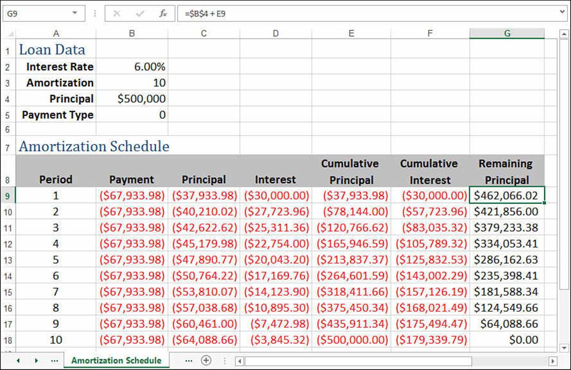
Figure 18.6 This worksheet shows a basic amortization schedule for a fixed-rate loan.
![]() The amortization schedule in Figure 18.6 assumes that the interest rate remains fixed throughout the life of the loan. To learn how to build an amortization schedule for a variable-rate loan, see “Building a Variable-Rate Mortgage Amortization Schedule,” p. 447.
The amortization schedule in Figure 18.6 assumes that the interest rate remains fixed throughout the life of the loan. To learn how to build an amortization schedule for a variable-rate loan, see “Building a Variable-Rate Mortgage Amortization Schedule,” p. 447.
Building a Dynamic Amortization Schedule
The problem with the amortization schedule in Figure 18.6 is that it’s static. It works well if you change the interest rate or the principal, but it doesn’t handle other types of changes very well:
![]() If you want to use a different time basis—for example, monthly instead of annual—you need to edit the initial formulas for payment, principal, interest, cumulative principal, and cumulative interest, and then refill the schedule.
If you want to use a different time basis—for example, monthly instead of annual—you need to edit the initial formulas for payment, principal, interest, cumulative principal, and cumulative interest, and then refill the schedule.
![]() If you want to use a different number of periods, you need to either extend the schedule (for a longer term) or shorten the schedule and delete the extraneous periods (for a shorter term).
If you want to use a different number of periods, you need to either extend the schedule (for a longer term) or shorten the schedule and delete the extraneous periods (for a shorter term).
Both operations are tedious and time-consuming enough that they greatly reduce the value of the amortization schedule. To make the schedule truly useful, you need to reconfigure it so that the schedule formulas and the schedule itself adjust automatically to any change in the time basis or the length of the term.
Figure 18.7 shows a worksheet that implements such a dynamic amortization schedule.
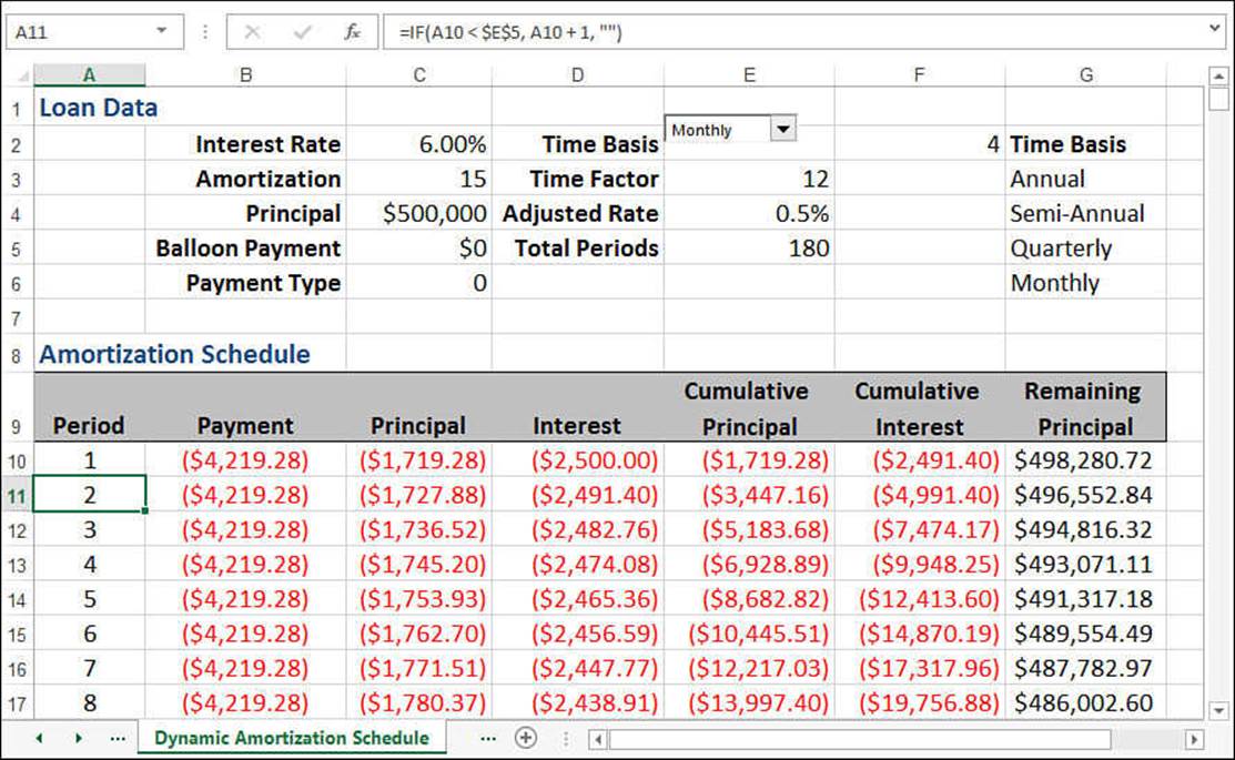
Figure 18.7 This worksheet uses a dynamic amortization schedule that adjusts automatically to changing the time basis or the length of the term.
Here’s a summary of the changes you make to create this schedule’s dynamic 'margin-top:4.0pt;margin-right:0cm;margin-bottom:4.0pt; margin-left:40.0pt;text-indent:-9.5pt;line-height:normal'>![]() To change the time basis, select a value—Annual, Semiannual, Quarterly, or Monthly—in the Time Basis drop-down list. These values come from the text literals in the range G3:G6. The number of the selected list item is stored in cell F2.
To change the time basis, select a value—Annual, Semiannual, Quarterly, or Monthly—in the Time Basis drop-down list. These values come from the text literals in the range G3:G6. The number of the selected list item is stored in cell F2.
![]() To learn how to add a list box to a worksheet, see “Using Dialog Box Controls on a Worksheet,” p. 103.
To learn how to add a list box to a worksheet, see “Using Dialog Box Controls on a Worksheet,” p. 103.
![]() The time basis determines the time factor, the amount by which you have to adjust the rate and the term. For example, if the time basis is Monthly, the time factor is 12. This means that you divide the annual interest rate (C2) by 12, and you multiply the term (C3) by 12. These new values are stored in the Adjusted Rate (E4) and Total Periods (E5) cells. The Time Factor cell (E3) uses the following formula:
The time basis determines the time factor, the amount by which you have to adjust the rate and the term. For example, if the time basis is Monthly, the time factor is 12. This means that you divide the annual interest rate (C2) by 12, and you multiply the term (C3) by 12. These new values are stored in the Adjusted Rate (E4) and Total Periods (E5) cells. The Time Factor cell (E3) uses the following formula:
=CHOOSE(F2, 1, 2, 4, 12)
![]() Given the adjusted rate (E4) and the total periods (E5), the schedule formulas can reference these cells directly and always return the correct value for any selected time basis. For example, here’s the expression that calculates the payment:
Given the adjusted rate (E4) and the total periods (E5), the schedule formulas can reference these cells directly and always return the correct value for any selected time basis. For example, here’s the expression that calculates the payment:
PMT(E4, E5, C4, C5, C6)
![]() The schedule adjusts its size automatically, depending on the Total Periods value (E5). If Total Periods is 15, the schedule contains 15 rows (not including the headers); if Total Periods is 180, the schedule contains 180 rows.
The schedule adjusts its size automatically, depending on the Total Periods value (E5). If Total Periods is 15, the schedule contains 15 rows (not including the headers); if Total Periods is 180, the schedule contains 180 rows.
![]() Dynamically adjusting the size of the schedule is a function of the Total Periods value (E5). The first period (A10) is always 1; each subsequent period checks the previous value to see if it’s less than Total Periods. Here’s the formula in cell A11:
Dynamically adjusting the size of the schedule is a function of the Total Periods value (E5). The first period (A10) is always 1; each subsequent period checks the previous value to see if it’s less than Total Periods. Here’s the formula in cell A11:
=IF(A10 < $E$5, A10 + 1, "")
If the period value of the cell above the current cell is less than Total Periods, the current cell is still within the schedule, so calculate the current period (the value from the cell above plus 1) and display the result; otherwise, you’ve gone past the end of the schedule, so display a blank.
![]() The various payment columns check the period value. If it’s not blank, calculate and display the result; otherwise, display a blank. Here’s the formula for the Payment value in B11:
The various payment columns check the period value. If it’s not blank, calculate and display the result; otherwise, display a blank. Here’s the formula for the Payment value in B11:
=IF(A11 <> "", PMT($E$4, $E$5, $C$4, $C$5, $C$6), "")
These changes result in a totally dynamic schedule that adjusts automatically as you change the time basis or the term.
Note
The formulas in the amortization schedule have been filled down to row 500, which should be enough room for just about any schedule (up to about 40 years, using the monthly basis). If you require a longer schedule, you’ll have to fill in the schedule formulas past the last row that will appear in your schedule.
Calculating the Term of a Loan
In some loan scenarios, you need to borrow a certain amount at the current interest rates, but you can spend only so much on each payment. If the other loan factors are fixed, the only way to adjust the payment is to adjust the term of the loan: A longer term means smaller payments; a shorter term means larger payments.
You could figure out the term by adjusting the nper argument of the PMT() function until you get the payment you want. However, Excel offers a more direct solution in the form of the NPER() function, which returns the number of periods of a loan:
NPER(rate, pmt, pv[, fv][, type])
For example, suppose that you want to borrow $10,000 at 6% interest with no balloon payment, and the most you can spend is $750 per month. What term should you get? Figure 18.8 shows a worksheet that uses NPER() to calculate the answer: 13.8 months. Here are some things to note about this model:
![]() The interest rate is an annual value, so the NPER() function’s rate argument divides the rate by 12.
The interest rate is an annual value, so the NPER() function’s rate argument divides the rate by 12.
![]() The payment is already a monthly number, so no adjustment is necessary for the pmt attribute.
The payment is already a monthly number, so no adjustment is necessary for the pmt attribute.
![]() The payment is negative because it’s money that you pay to the lender.
The payment is negative because it’s money that you pay to the lender.
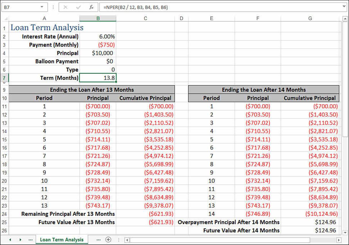
Figure 18.8 This worksheet uses NPER() to determine the number of months that a $10,000 loan should be taken out at 6% interest to ensure a monthly payment of $750.
Of course, in the real world, although it’s not unusual to have a noninteger term, the last payment must occur at the beginning or end of the last loan period. In the example, the bank uses the term 13.8 months to calculate the payment, principal, and interest, but it rightly insists that the last payment be made at either the 13th period or the 14th period. The tables after the NPER() formula in Figure 18.8 investigate both scenarios.
If you elect to end the loan after the 13th period, you’ll still have a bit of principal left over. To see why, the amortization table shows the period (column A) as well as the principal paid each period (column B), as returned by the PPMT() function. The Cumulative Principal column (column C) shows a running total of the principal. As you can see, after 13 months, the total principal paid is only $9,378.07, which leaves $621.93 remaining (cell C24). Therefore, the 13th payment will be $1,371.93 (the usual $750 payment, plus the remaining $621.93 principal).
Note
The cumulative principal values are calculated using the SUM() function. You can’t use the CUMPRINC() function in this case because CUMPRINC() truncates the nper argument to an integer value.
If you elect to end the loan after the 14th period instead, you’ll end up overpaying the principal. To see why, the second amortization table shows the Period (column E), Principal (column F), and Cumulative Principal (column G) columns. After 14 months, the total principal paid is $10,124.96, which is $124.96 more than the original $10,000 principal. Therefore, the 14th payment will be $625.04 (the usual $750 payment minus the $124.96 principal overpayment).
Note
Another way to calculate the principal that is left over or overpaid is to use the FV() function, which returns the future value of a series of payments. For the 13-month scenario, you run FV() with the nper argument set to 13 (see cell C25 in Figure 18.8); for the 14-month scenario, you run FV() with the nper argument set to 14 (see cell G26). You’ll learn about FV() in detail in Chapter 19.
Calculating the Interest Rate Required for a Loan
A slightly less common loan scenario arises when you know the loan term, payment, and principal, and you need to know what interest rate will satisfy these parameters. This is useful in a number of circumstances:
![]() You might want to wait until interest rates fall to the value you want.
You might want to wait until interest rates fall to the value you want.
![]() You might regard the calculated interest rate as a maximum rate that you can pay, knowing that anything less will enable you to reduce either the payment or the term.
You might regard the calculated interest rate as a maximum rate that you can pay, knowing that anything less will enable you to reduce either the payment or the term.
![]() You could use the calculated interest rate as a negotiating tool with your lender by asking for that rate and walking away from the deal if you don’t get it.
You could use the calculated interest rate as a negotiating tool with your lender by asking for that rate and walking away from the deal if you don’t get it.
To determine the interest rate given the other loan factors, use the RATE() function:
RATE(nper, pmt, pv[, fv][, type][, guess])

![]() The RATE() function’s guess argument indicates that this function uses iteration to determine the answer. To learn more about iteration, see “Using Iteration and Circular References,” p. 93.
The RATE() function’s guess argument indicates that this function uses iteration to determine the answer. To learn more about iteration, see “Using Iteration and Circular References,” p. 93.
For example, suppose you want to borrow $10,000 over five years with no balloon payment and a monthly payout of $200. What rate will satisfy these criteria? The worksheet in Figure 18.9 uses RATE() to derive the result: 7.4%. Here are some notes about this model:
![]() The term is in years, so the RATE() function’s nper argument multiplies the term by 12.
The term is in years, so the RATE() function’s nper argument multiplies the term by 12.
![]() The payment is already a monthly number, so no adjustment is necessary for the pmt attribute.
The payment is already a monthly number, so no adjustment is necessary for the pmt attribute.
![]() The payment is negative because it’s money that you pay to the lender.
The payment is negative because it’s money that you pay to the lender.
![]() The result of the RATE() function is multiplied by 12 to get the annual interest rate.
The result of the RATE() function is multiplied by 12 to get the annual interest rate.
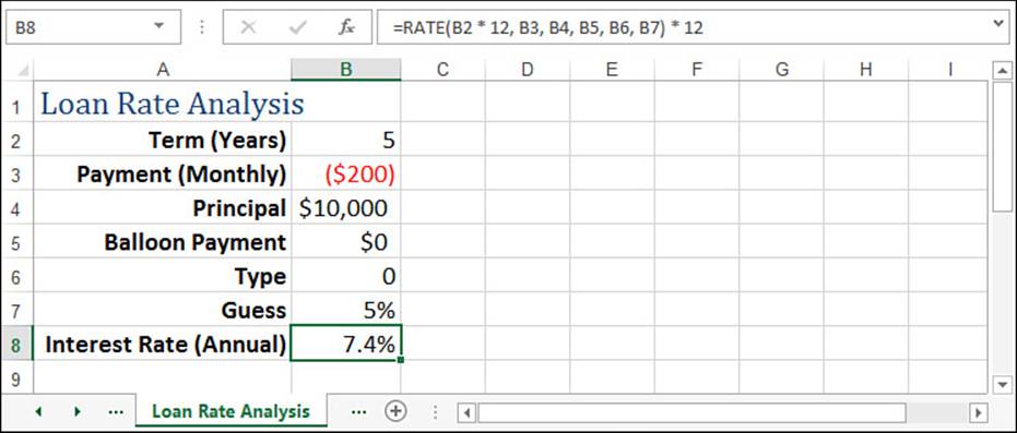
Figure 18.9 This worksheet uses RATE() to determine the interest rate required to pay a $10,000 loan over five years at $200 per month.
Calculating How Much You Can Borrow
If you know the current interest rate your bank is offering for loans, when you want to have the loan paid off, and how much you can afford each month for the payments, you might then wonder what is the maximum amount you can borrow under those terms. To figure this out, you need to solve for the principal—that is, present value. You do this in Excel by using the PV() function:
PV(rate, nper, pmt[, fv][, type])
For example, suppose the current loan rate is 6%, you want the loan paid off in five years, and you can afford payments of $500 per month. Figure 18.10 shows a worksheet that calculates the maximum amount you can borrow—$25,862.78—using the following formula:
=PV(B2 / 12, B3 * 12, B4, B5, B6)
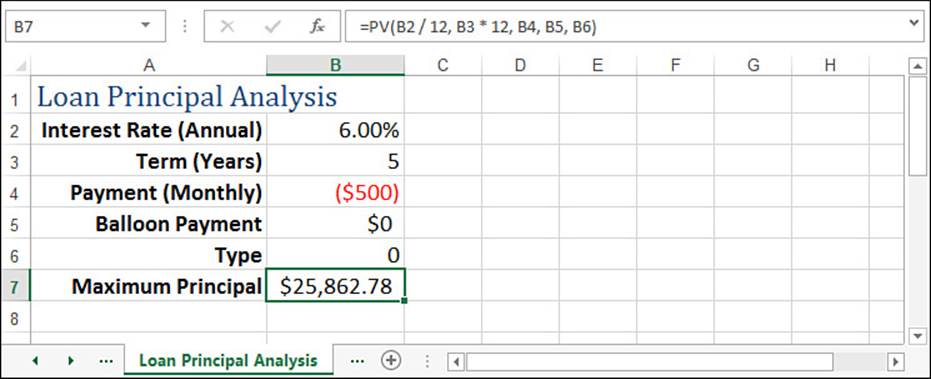
Figure 18.10 This worksheet uses PV() to calculate the maximum principal you can borrow, given a fixed interest rate, term, and monthly payment.
Case Study: Working with Mortgages
For both businesses and people, a mortgage is almost always the largest financial transaction. Whether it’s millions of dollars for a new building or hundreds of thousands of dollars for a house, a mortgage is serious business. It pays to know exactly what you’re getting into, both in terms of long-term cash flow and in terms of making good decisions up front about the type of mortgage so that you minimize your interest costs. This case study takes a look at mortgages from both points of view.
Building a Variable-Rate Mortgage Amortization Schedule
For simplicity’s sake, it’s possible to build a mortgage amortization schedule like the ones shown earlier in this chapter. However, these are not always realistic because a mortgage rarely uses the same interest rate over the full amortization period. Instead, you usually have a fixed rate over a specific term (usually one to five years), and you then renegotiate the mortgage for a new term. This renegotiation involves changing three things:
![]() The interest rate over the coming term, which will reflect current market rates.
The interest rate over the coming term, which will reflect current market rates.
![]() The amortization period, which will now be shorter by the length of the previous term. For example, a 25-year amortization will drop to a 20-year amortization after a 5-year term.
The amortization period, which will now be shorter by the length of the previous term. For example, a 25-year amortization will drop to a 20-year amortization after a 5-year term.
![]() The present value of the mortgage, which will be the remaining principal at the end of the term.
The present value of the mortgage, which will be the remaining principal at the end of the term.
Figure 18.11 shows an amortization schedule that takes these mortgage realities into account.
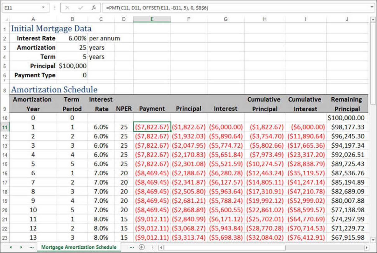
Figure 18.11 A mortgage amortization schedule that reflects the changing interest rates, amortization periods, and present value at each new term.
Here’s a summary of what’s happening with each column in the amortization:
![]() Amortization Year—This column gives the year of the overall amortization. This is mainly used to help calculate the Term Period values. Note that the values in this column are generated automatically based on the value in the Amortization (Years) cell (B3).
Amortization Year—This column gives the year of the overall amortization. This is mainly used to help calculate the Term Period values. Note that the values in this column are generated automatically based on the value in the Amortization (Years) cell (B3).
![]() Term Period—This column gives the year of the current term. This is a calculated value (it uses the MOD() function) based on the value in the Amortization Year column and the value in the Term (Years) cell (B4).
Term Period—This column gives the year of the current term. This is a calculated value (it uses the MOD() function) based on the value in the Amortization Year column and the value in the Term (Years) cell (B4).
![]() Interest Rate—This is the interest rate applied to each term. You enter these rates by hand.
Interest Rate—This is the interest rate applied to each term. You enter these rates by hand.
![]() NPER—This is the amortization period applied to each term. It’s used as the nper argument for the PMT(), PPMT(), and IPMT() functions. You enter these values by hand.
NPER—This is the amortization period applied to each term. It’s used as the nper argument for the PMT(), PPMT(), and IPMT() functions. You enter these values by hand.
![]() Payment—This is the monthly payment for the current term. The PMT() function uses the Interest Rate column value for the rate argument and the NPER column value for the nper argument. For the pv argument, the function grabs the remaining balance at the end of the previous term by using the OFFSET() function in the following general form:
Payment—This is the monthly payment for the current term. The PMT() function uses the Interest Rate column value for the rate argument and the NPER column value for the nper argument. For the pv argument, the function grabs the remaining balance at the end of the previous term by using the OFFSET() function in the following general form:
OFFSET(current_cell, -Term_Period, 5)
In this formula, current_cell is a reference to the cell containing the formula, and Term_Period is a reference to the corresponding cell in the Term Period column. For example, here’s the formula in E11:
OFFSET(E11, -B11, 5)
Because the value in B11 is 1, the function goes up one row and right five columns, which returns the value in J10 (in this case, the original principal).
![]() Principal and Interest—These columns calculate the principal and interest components of the payment, and they use the same techniques as the Payment column.
Principal and Interest—These columns calculate the principal and interest components of the payment, and they use the same techniques as the Payment column.
![]() Cumulative Principal and Cumulative Interest—These columns calculate the total principal and interest paid through the end of each year. Because the interest rate isn’t constant over the life of the loan, you can’t use CUMPRINC() and CUMIPMT(). Instead, these columns use running SUM() functions.
Cumulative Principal and Cumulative Interest—These columns calculate the total principal and interest paid through the end of each year. Because the interest rate isn’t constant over the life of the loan, you can’t use CUMPRINC() and CUMIPMT(). Instead, these columns use running SUM() functions.
![]() Remaining Principal—This column calculates the principal left on the loan by subtracting the value in the Principal column for each year. At the end of each term, the Remaining Principal value is used as the pv argument in the PMT(), PPMT(), and IPMT() functions over the next term. In Figure 18.11, for example, at the end of the first five-year term, the remaining principal is $89,725.43, so that’s the present value used throughout the second five-year term.
Remaining Principal—This column calculates the principal left on the loan by subtracting the value in the Principal column for each year. At the end of each term, the Remaining Principal value is used as the pv argument in the PMT(), PPMT(), and IPMT() functions over the next term. In Figure 18.11, for example, at the end of the first five-year term, the remaining principal is $89,725.43, so that’s the present value used throughout the second five-year term.
Allowing for Mortgage Principal Paydowns
Many mortgages today allow you to include in each payment an extra amount that goes directly to paying down the mortgage principal. Before you decide to take on the financial burden of these extra paydowns, you probably want two questions answered:
![]() How much more quickly will I pay off the mortgage?
How much more quickly will I pay off the mortgage?
![]() How much money will I save over the amortization period?
How much money will I save over the amortization period?
Both questions are easily answered using Excel’s financial functions. Consider the mortgage-analysis model I’ve set up in Figure 18.12. The Initial Mortgage Data area shows the basic numbers needed for the calculations: the annual interest rate (cell B2), the amortization period (B3), the principal (B4), and the paydown that is to be added to each payment (B5; notice that this is a negative number because it represents a monetary outflow).
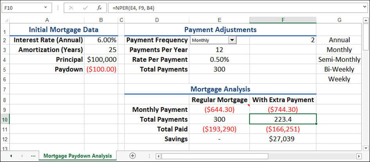
Figure 18.12 A mortgage-analysis worksheet that calculates the effect of making extra monthly paydowns toward the principal.
The Payment Adjustments area contains four values:
![]() Payment Frequency—Use this drop-down list to specify how often you make your mortgage payments. The available values—Annual, Monthly, Semi-Monthly, Bi-Weekly, and Weekly—come from the range G2:G6; the number of the selected list item is stored in cell F2.
Payment Frequency—Use this drop-down list to specify how often you make your mortgage payments. The available values—Annual, Monthly, Semi-Monthly, Bi-Weekly, and Weekly—come from the range G2:G6; the number of the selected list item is stored in cell F2.
![]() Payments Per Year (E3)—This is the number of payments per year, as given by the following formula:
Payments Per Year (E3)—This is the number of payments per year, as given by the following formula:
=CHOOSE(F2, 1, 12, 24, 26, 52)
![]() Rate Per Payment—This is the annual rate divided by the number of payments per year.
Rate Per Payment—This is the annual rate divided by the number of payments per year.
![]() Total Payments—This is the amortization value multiplied by the number of payments per year.
Total Payments—This is the amortization value multiplied by the number of payments per year.
The Mortgage Analysis area shows the results of various calculations:
![]() Frequency Payment (Frequency is the selected item in the drop-down list.)—The Regular Mortgage payment (E9) is calculated using the PMT() function, where the rate argument is the Rate Per Payment value (E4) and the nper argument is the Total Payments value (E5):
Frequency Payment (Frequency is the selected item in the drop-down list.)—The Regular Mortgage payment (E9) is calculated using the PMT() function, where the rate argument is the Rate Per Payment value (E4) and the nper argument is the Total Payments value (E5):
=PMT(E4, E5, B4, 0, 0)
The With Extra Payment value (F9) is the sum of the Paydown (B5) and the Regular Mortgage payment (E9).
![]() Total Payments—For the Regular Mortgage (E10), this is the same as the Total Payments value (E5). It’s copied here to make it easy for you to compare this value with the With Extra Payment value (F10), which calculates the revised term with the extra paydown included. It does this with the NPER() function, where the rate argument is the Rate Per Payment value (E4) and the pmt argument is the payment in the With Extra Payment column (F9).
Total Payments—For the Regular Mortgage (E10), this is the same as the Total Payments value (E5). It’s copied here to make it easy for you to compare this value with the With Extra Payment value (F10), which calculates the revised term with the extra paydown included. It does this with the NPER() function, where the rate argument is the Rate Per Payment value (E4) and the pmt argument is the payment in the With Extra Payment column (F9).
![]() Total Paid—These values multiply the Payment value by the Total Payments value for each column.
Total Paid—These values multiply the Payment value by the Total Payments value for each column.
![]() Savings—This value (cell F12) takes the difference between the Total Paid values to show how much money you save by including the paydown in each payment.
Savings—This value (cell F12) takes the difference between the Total Paid values to show how much money you save by including the paydown in each payment.
In the example shown in Figure 18.12, paying an extra $100 per month toward the mortgage principal reduces the term on a $100,000 mortgage from 300 months (25 years) to 223.4 months (about 18.5 years) and reduces the total amount paid from $193,290 to $166,251, a savings of $27,039.
From Here
![]() To learn how to add a list box to a worksheet, see “Using Dialog Box Controls on a Worksheet,” p. 103.
To learn how to add a list box to a worksheet, see “Using Dialog Box Controls on a Worksheet,” p. 103.
![]() The RATE() function uses iteration to calculate its value. To learn more about iteration, see “Using Iteration and Circular References,” p. 83.
The RATE() function uses iteration to calculate its value. To learn more about iteration, see “Using Iteration and Circular References,” p. 83.
![]() Many of the functions you learned in this chapter—including PMT(), RATE(), and NPER()—can also be used with investment calculations. See Chapter 19, “Building Investment Formulas,” p. 453.
Many of the functions you learned in this chapter—including PMT(), RATE(), and NPER()—can also be used with investment calculations. See Chapter 19, “Building Investment Formulas,” p. 453.
![]() The PV() function is most often used in discount calculations. See “Calculating the Present Value,” p. 468.
The PV() function is most often used in discount calculations. See “Calculating the Present Value,” p. 468.
All materials on the site are licensed Creative Commons Attribution-Sharealike 3.0 Unported CC BY-SA 3.0 & GNU Free Documentation License (GFDL)
If you are the copyright holder of any material contained on our site and intend to remove it, please contact our site administrator for approval.
© 2016-2026 All site design rights belong to S.Y.A.