Excel® 2016 Formulas and Functions (2016)

Part IV: Building Financial Formulas

19. Building Investment Formulas

In This Chapter

Working with Interest Rates

Calculating the Future Value

Working Toward an Investment Goal

The time value of money concepts introduced in Chapter 18, “Building Loan Formulas,” applies equally well to investments. The only difference is that you need to reverse the signs of the cash values. That’s because loans generally involve receiving a principal amount (positive cash flow) and paying it back over time (negative cash flow). An investment, on the other hand, involves depositing money into the investment (negative cash flow) and then receiving interest payments (or whatever) in return (positive cash flow).

With this sign change in mind, this chapter takes you through some Excel tools for building investment formulas. You’ll learn about the wonders of compound interest; how to convert between nominal and effective interest rates; how to calculate the future value of an investment; ways to work toward an investment goal by calculating the required interest rate, term, and deposits; and how to build an investment schedule.

Working with Interest Rates

As I mentioned in Chapter 18, the interest rate is the mechanism that transforms a present value into a future value. (Or, operating as a discount rate, it’s what transforms a future value into a present value.) Therefore, when working with financial formulas, it’s important to know how to work with interest rates and to be comfortable with certain terminology. You’ve already seen (again, in Chapter 18) that it’s crucial for the interest rate, term, and payment to use the same time basis. The next sections show you a few other interest rate techniques you should know.

Understanding Compound Interest

An interest rate is described as simple if it pays the same amount each period. For example, if you have $1,000 in an investment that pays a simple interest rate of 10% per year, you’ll receive $100 each year.

Suppose, however, that you were able to add the interest payments to the investment. At the end of the first year, you would have $1,100 in the account, which means you would earn $110 in interest (10% of $1,100) the second year. Being able to add interest earned to an investment is calledcompounding, and the total interest earned (the normal interest plus the extra interest on the reinvested interest—the extra $10, in the example) is called compound interest.

Nominal Versus Effective Interest

Interest can also be compounded within the year. For example, suppose that your $1,000 investment earns 10% compounded semiannually. At the end of the first six months, you receive $50 in interest (5% of the original investment). This $50 is reinvested, and for the second half of the year, you earn 5% of $1,050, or $52.50. Therefore, the total interest earned in the first year is $102.50. In other words, the interest rate appears to actually be 10.25%. So which is the correct interest rate, 10% or 10.25%?

To answer that question, you need to know about the two ways that most interest rates are most often quoted:

The nominal rate—This is the annual rate before compounding (the 10% rate, in the example). The nominal rate is always quoted along with the compounding frequency—for example, 10% compounded semiannually.

Note

The nominal annual interest rate is often shortened to APR, or the annual percentage rate.

The effective rate—This is the annual rate that an investment actually earns in the year after the compounding is applied (the 10.25%, in the example).

In other words, both rates are “correct,” except that, with the nominal rate, you also need to know the compounding frequency.

If you know the nominal rate and the number of compounding periods per year (for example, semiannually means 2 compounding periods per year, and monthly means 12 compounding periods per year), you get the effective rate per period by dividing the nominal rate by the number of periods:

=nominal_rate / npery

Here, npery is the number of compounding periods per year. To convert the nominal annual rate into the effective annual rate, you use the following formula:

=(1 + nominal_rate / npery) ^ npery - 1

Conversely, if you know the effective rate per period, you can derive the nominal rate by multiplying the effective rate by the number of periods:

=effective_rate * npery

To convert the effective annual rate to the nominal annual rate, you use the following formula:

=npery * (effective_rate + 1) ^ (1 / npery) - npery

Fortunately, the next section shows you two functions that can handle the conversion between the nominal and effective annual rates for you.

Converting Between the Nominal Rate and the Effective Rate

To convert a nominal annual interest rate to the effective annual rate, use the EFFECT() function:

EFFECT(nominal_rate, npery)

For example, the following formula returns the effective annual interest rate for an investment with a nominal annual rate of 10% that compounds semiannually:

=EFFECT(0.1, 2)

Figure 19.1 shows a worksheet that applies the EFFECT() function to a 10% nominal annual rate using various compounding frequencies.

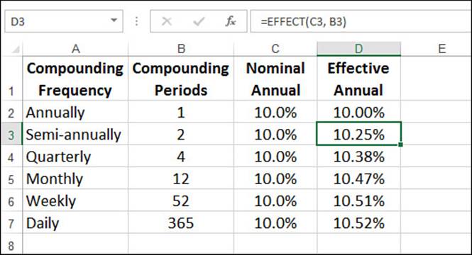
Figure 19.1 The formulas in column D use the EFFECT() function to convert the nominal rates in column C to effective rates based on the compounding periods in column B.

Note

You can download the workbook that contains this chapter’s examples at www.mcfedries.com/books/book.php?title=excel-2016-formulas-and-functions.

If you already know the effective annual interest rate and the number of compounding periods, you can convert the rate to the nominal annual interest rate by using the NOMINAL() function:

NOMINAL(effect_rate, npery)

For example, the following formula returns the nominal annual interest rate for an investment with an effective annual rate of 10.52% that compounds daily:

=NOMINAL(0.1052, 365)

Calculating the Future Value

Just as the payment is usually the most important value for a loan calculation, the future value is usually the most important value for an investment calculation. After all, the purpose of an investment is to place a sum of money (the present value) in some instrument for a time, after which you end up with some new (and hopefully greater) amount: the future value.

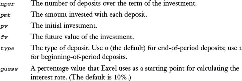
To calculate the future value of an investment, Excel offers the FV() function:

FV(rate, nper[, pmt][, pv][, type])

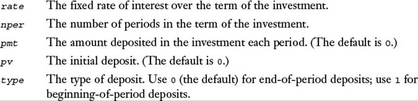
Because both the amount deposited per period (the pmt argument) and the initial deposit (the pv argument) are sums that you pay out, these must be entered as negative values in the FV() function.

The next few sections take you through various investment scenarios using the FV() function.

The Future Value of a Lump Sum

In the simplest future value scenario, you invest a lump sum and let it grow according to the specified interest rate and term, without adding any deposits along the way. In this case, you use the FV() function with the pmt argument set to 0:

FV(rate, nper, 0, pv, type)

For example, Figure 19.2 shows the future value of $10,000 invested at 5% over 10 years.

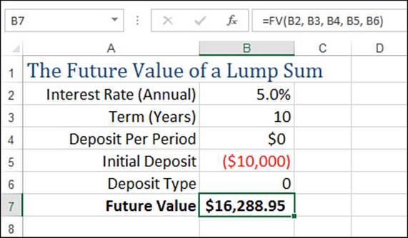
Figure 19.2 When calculating the future value of an initial lump sum deposit, set the FV() function’s pmt argument to 0.

Tip

Excel’s FV() function doesn’t work with continuous compounding. Instead, you need to use a worksheet formula that takes the following general form (where e is the mathematical constant e):

=pv * e ^ (rate * nper)

For example, the following formula calculates the future value of $10,000 invested at 5% over 10 years compounded continuously (and it returns a value of $16,487.21):

=10000 * EXP(0.05 * 10)

The Future Value of a Series of Deposits

Another common investment scenario is to make a series of deposits over the term of the investment, without depositing an initial sum. In this case, you use the FV() function with the pv argument set to 0:

FV(rate, nper, pmt, 0, type)

For example, Figure 19.3 shows the future value of $100 invested each month at 5% over 10 years. Notice that the interest rate and term are both converted to monthly amounts because the deposit occurs monthly.

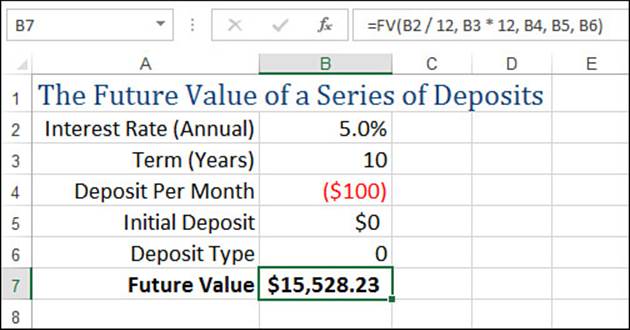
Figure 19.3 When calculating the future value of a series of deposits, set the FV() function’s pv argument to 0.

The Future Value of a Lump Sum Plus Deposits

For best investment results, you should invest an initial amount and then add to it with regular deposits. In this scenario, you need to specify all the FV() function arguments (except type). For example, Figure 19.4 shows the future value of an investment with a $10,000 initial deposit and $100 monthly deposits at 5% over 10 years.

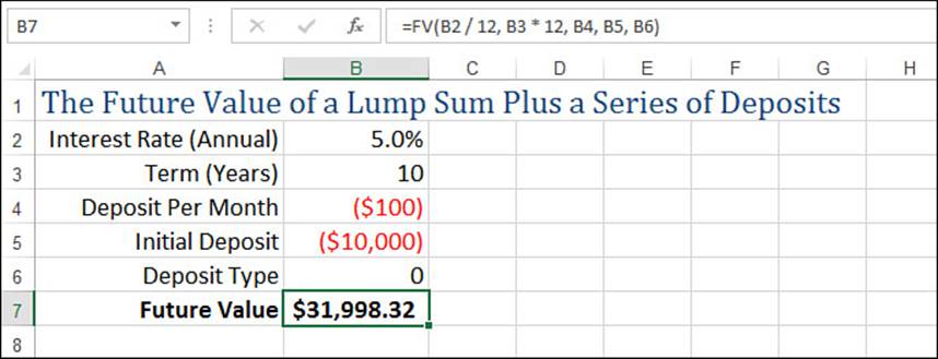
Figure 19.4 This worksheet uses the full FV() function syntax to calculate the future value of a lump sum plus a series of deposits.

Working Toward an Investment Goal

Instead of just seeing where an investment will end up, it’s often desirable to have a specific monetary goal in mind and then ask yourself, “What will it take to get me there?”

Answering this question means solving for one of the four main future value parameters—interest rate, number of periods, regular deposit, and initial deposit—while holding the other parameters (and, of course, your future value goal) constant. The next four sections take you through this process.

Calculating the Required Interest Rate

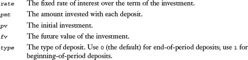
Say that you know the future value that you want, when you want it, and the initial deposit and periodic deposits you can afford. What interest rate do you require to meet your goal? You answer this question by using the RATE() function, which you first encountered in Chapter 18. Here’s the syntax for that function from the point of view of an investment:

RATE(nper, pmt, pv, fv[, type][, guess])

For example, if you need $100,000 10 years from now, you are starting with $10,000, and you can deposit $500 per month. What interest rate is required to meet your goal? Figure 19.5 shows a worksheet that comes up with the answer: 6%.

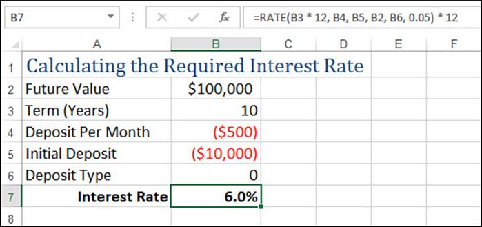
Figure 19.5 Use the RATE() function to work out the interest rate required to reach a future value, given a fixed term, a periodic deposit, and an initial deposit.

To work with the RATE() function in a loan context, see “Calculating the Interest Rate Required for a Loan,” p. 445.

Calculating the Required Number of Periods

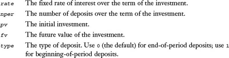
Given your investment goal, if you have an initial deposit and an amount that you can afford to deposit periodically, how long will it take to reach your goal at the prevailing market interest rate? You answer this question by using the NPER() function (which was introduced in Chapter 18). Here’s the NPER() syntax from the point of view of an investment:

NPER(rate, pmt, pv, fv[, type])

For example, suppose that you want to retire with $1,000,000. You have $50,000 to invest, you can afford to deposit $1,000 per month, and you expect to earn 5% interest. How long will it take to reach your goal? The worksheet in Figure 19.6 answers this question: 349.4 months, or 29.1 years.

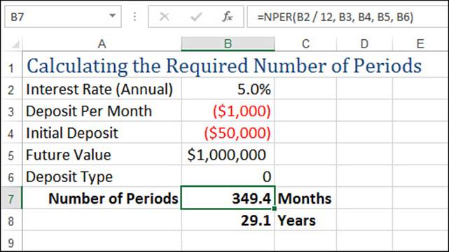
Figure 19.6 Use the NPER() function to calculate how long it will take to reach a future value, given a fixed interest rate, a periodic deposit, and an initial deposit.

To work with the NPER() function in a loan context, see “Calculating the Term of a Loan,” p. 443.

Calculating the Required Regular Deposit

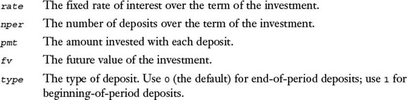
Suppose that you want to reach your future value goal by a certain date and that you have an initial amount to invest. Given current interest rates, how much extra do you have to periodically deposit into the investment to achieve your goal? The answer here lies in the PMT() function fromChapter 18. Here are the PMT() function details from the point of view of an investment:

PMT(rate, nper, pv, fv[, type])

For example, suppose you want to end up with $50,000 in 15 years to finance your child’s college education. If you have no initial deposit and you expect to get 7.5% interest over the term of the investment, how much do you need to deposit each month to reach your target? Figure 19.7shows a worksheet that calculates the result using PMT(): $151.01 per month.

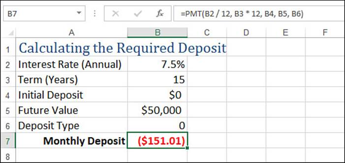
Figure 19.7 Use the PMT() function to derive how much you need to deposit periodically to reach a future value, given a fixed interest rate, a number of deposits, and an initial deposit.

To work with the PMT() function in a loan context, see “Calculating a Loan Payment,” p. 435.

Calculating the Required Initial Deposit

For the final standard future value calculation, suppose that you know when you want to reach your goal, how much you can deposit each period, and how much the interest rate will be. What, then, do you need to deposit initially to achieve your future value target? To find the answer, you use the PV() function. Here are the PV() function details from the point of view of an investment:

PV(rate, nper, pmt, fv[, type])

For example, suppose your goal is to end up with $100,000 in three years to purchase new equipment. If you expect to earn 6% interest and can deposit $2,000 monthly, what does your initial deposit have to be to make your goal? The worksheet in Figure 19.8 uses PV() to calculate the answer: $17,822.46.

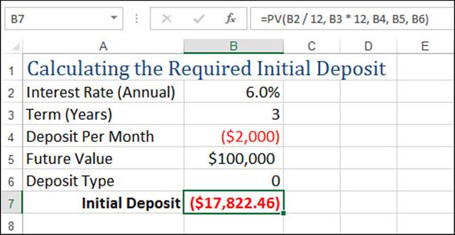
Figure 19.8 Use the PV() function to find out how much you need to deposit initially to reach a future value, given a fixed interest rate, number of deposits, and periodic deposit.

To work with the PV() function in a discount context, see “Calculating the Present Value,” p. 468.

Calculating the Future Value with Varying Interest Rates

All the future value examples that you’ve worked with so far have assumed that the interest rate remained constant over the term of the investment. This will always be true for fixed-rate investments, but for other investments, such as mutual funds, stocks, and bonds, using a fixed rate of interest is, at best, a guess about what the average rate will be over the term.

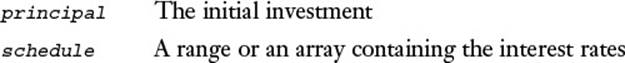
For investments that offer a variable rate over the term, or when the rate fluctuates over the term, Excel offers the FVSCHEDULE() function, which returns the future value of some initial amount, given a schedule of interest rates:

FVSCHEDULE(principal, schedule)

For example, the following formula returns the future value of an initial $10,000 deposit that makes 5%, 6%, and 7% over three years:

=FVSCHEDULE(10000, {0.05, 0.06, 0.07})

Similarly, Figure 19.9 shows a worksheet that calculates the future value of an initial deposit of $100,000 into an investment that earns 5%, 5.5%, 6%, 7%, and 6% over five years.

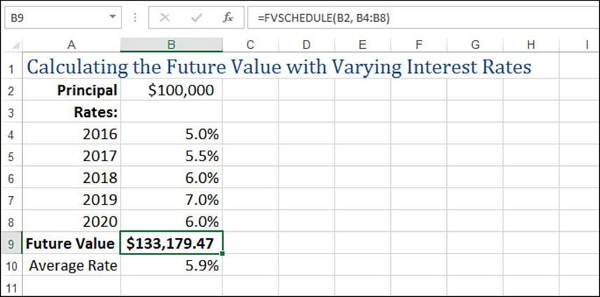
Figure 19.9 Use the FVSCHEDULE() function to return the future value of an initial deposit in an investment that earns varying rates of interest.

Note

If you want to know the average rate earned on the investment, use the RATE() function, where nper is the number of values in the interest rate schedule, pmt is 0, pv is the initial deposit, and fv is the negative of the FVSCHEDULE() result. Here’s the general syntax:

RATE(ROWS(schedule), 0, principal, -FVSCHEDULE(principal,
schedule))

Case Study: Building an Investment Schedule

If you’re planning future cash-flow requirements or future retirement needs, it’s often not enough just to know how much money you’ll have at the end of an investment. You might need to also know how much money is in the investment account or fund at each period throughout the life of the investment.

To do this, you need to build an investment schedule. This is similar to an amortization schedule, except that it shows the future value of an investment at each period in the term of the investment.

To learn about amortization schedules, see “Building a Loan Amortization Schedule,” p. 440.

In a typical investment schedule, you need to take two things into account:

The periodic deposits put into the investment, particularly the amount deposited and the frequency of the deposits. The frequency of the deposits determines the total number of periods in the investment. For example, a 10-year investment with semiannual deposits has 20 periods.

The compounding frequency of the investment (annually, semiannually, and so on). Assuming that you know the APR (that is, nominal annual interest rate), you can use the compounding frequency to determine the effective rate.

Note, however, that you can’t simply use the EFFECT() function to convert the known nominal rate into the effective rate. That’s because you’re going to calculate the future value at the end of each period, which might or might not correspond to the compounding frequency. (For example, if the investment compounds monthly and you deposit semiannually, there will be six months of compounding to factor into the future value at the end of each period.)

Getting the proper effective rate for each period requires three steps:

1. Use the EFFECT() function to convert the nominal annual rate into the effective annual rate, based on the compounding frequency.

2. Use the NOMINAL() function to convert the effective rate from step 1 into the nominal rate, based on the deposit frequency.

3. Divide the nominal rate from step 2 by the deposit frequency to get the effective rate per period. This is the value that you’ll plug in to the FV() function.

Figure 19.10 shows a worksheet that implements an investment schedule using this technique.

Figure 19.10 An investment schedule that takes into account deposit frequency and compounding frequency to return the future value of an investment at the end of each deposit period.

Here’s a summary of the items in the Investment Data portion of the worksheet:

Nominal Rate (APR) (B2)—This is the nominal annual rate of interest for the investment.

Term (Years) (B3)—This is the length of the investment, in years.

Initial Deposit (B4)—This is the amount deposited at the start of the investment. Enter this as a negative number (because it’s money that you’re paying out).

Periodic Deposit (B5)—This is the amount deposited at each period of the investment. (Again, this number must be negative.)

Deposit Type (B6)—This is the type argument of the FV() function.

Deposit Frequency—Use this drop-down list to specify how often the periodic deposits are made. The available values—Annually, Semi-Annually, Quarterly, Monthly, Weekly, and Daily—come from the range F2:F7; the number of the selected list item is stored in cell E2.

Deposits Per Year (D3)—This is the number of periods per year, as given by the following formula:

=CHOOSE(E2, 1, 2, 4, 12, 52, 365)

Compounding Frequency—Use this drop-down list to specify how often the investment compounds. You get the same options as in the Deposit Frequency list. The number of the selected list item is stored in cell E4.

Compounds Per Year (D5)—This is the number of compounding periods per year, as given by the following formula:

=CHOOSE(E4, 1, 2, 4, 12, 52, 365)

Effective Rate Per Period (D6)—This is the effective interest rate per period, as calculated using the three-step algorithm outlined earlier in this section. Here’s the formula:

=NOMINAL(EFFECT(B2, D5), D3) / D3

Total Periods (D7)—This is the total number of deposit periods in the loan, which is just the term multiplied by the number of deposits per year.

Here’s a summary of the columns in the Investment Schedule portion of the worksheet:

Period (column A)—This is the period number of the investment. The Period values are generated automatically based on the Total Periods value (D7).

The dynamic features used in the investment schedule are similar to those used in the dynamic amortization schedule; see “Building a Dynamic Amortization Schedule,” p. 441.

Interest Earned (column B)—This is the interest earned during the period. It’s calculated by multiplying the future value from the previous period by the Effective Rate Per Period (D6).

Cumulative Interest (column C)—This is the total interest earned in the investment at the end of each period. It’s calculated by using a running sum of the values in the Interest Earned column.

Cumulative Deposits (column D)—This is the total amount of the deposits added to the investment at the end of each period. It’s calculated by multiplying the Periodic Deposit (B5) by the current period number (column A).

Total Increase (column E)—This is the total amount by which the investment has increased over the Initial Deposit at the end of each period. It’s calculated by adding the Cumulative Interest and the Cumulative Deposits.

Future Value (column F)—This is the value of the investment at the end of each period. Here’s the FV() formula for cell F11:

=FV($D$6, A11, $B$5, $B$4, $B$6)

From Here

To get the details on the concept of the time value of money, see “Understanding the Time Value of Money,” p. 433.

To work with the RATE() function in a loan context, see “Calculating the Interest Rate Required for a Loan,” p. 445.

To work with the NPER() function in a loan context, see “Calculating the Term of a Loan,” p. 443.

To work with the PMT() function in a loan context, see “Calculating a Loan Payment,” p. 435.

To learn about amortization schedules, see “Building a Loan Amortization Schedule,” p. 440.

To work with the PV() function in a discount context, see “Calculating the Present Value,” p. 468.