Excel® 2016 Formulas and Functions (2016)
Part I: Mastering Excel Ranges and Formulas
5. Troubleshooting Formulas
In This Chapter
Understanding Excel’s Error Values
Fixing Other Formula Errors
Handling Formula Errors with IFERROR()
Using the Formula Error Checker
Auditing a Worksheet
Despite your best efforts, the odd error might appear in your formulas from time to time. Such errors can be mathematical (for example, dividing by zero), or Excel might simply be incapable of interpreting the formula. In the latter case, problems can be caught while you’re entering the formula. For example, if you try to enter a formula that has unbalanced parentheses, Excel won’t accept the entry, and it displays an error message. Other errors are more insidious. For example, your formula might appear to be working—that is, it might return a value—but the result may be incorrect because the data is flawed or because your formula has referenced the wrong cell or range.
Whatever the error and whatever the cause, formula woes need to be worked out because you or someone else in your company is likely depending on your models to produce accurate results. Don’t fall into the trap of thinking that your spreadsheets are problem free. A recent University of Hawaii study found that 50% of spreadsheets contained errors that led to “significant miscalculations.” And the more complex the model, the greater the chance that errors can creep in. A KPMG study from a few years ago found that a staggering 90% of spreadsheets used for tax calculations contained errors.
The good news is that fixing formula flaws need not be drudgery. With a bit of know-how and Excel’s top-notch troubleshooting tools, sniffing out and repairing model maladies isn’t hard. This chapter tells you everything you need to know.
Tip
If you try to enter an incorrect formula, Excel won’t let you do anything else until you either fix the problem or cancel the operation (which means you lose your formula). If the formula is complex, you might not be able to see the problem right away. Instead of deleting all your work, place an apostrophe (') at the beginning of the formula to convert it to text. This way, you can save your work while you try to figure out the problem.
Understanding Excel’s Error Values
When you enter or edit a formula or change one of the formula’s input values, Excel might show an error value as the formula result. Excel has seven different error values: #DIV/0!, #N/A, #NAME?, #NULL!, #NUM!, #REF!, and #VALUE!. The next few sections give you a detailed look at these error values and offer suggestions for dealing with them.
#DIV/0!
The #DIV/0! error almost always means that the cell’s formula is trying to divide by zero, a mathematical no-no. The cause is usually a reference to a cell that either is blank or contains the value 0. Check the cell’s precedents (the cells that are directly or indirectly referenced in the formula) to look for possible culprits. You’ll also see #DIV/0! if you enter an inappropriate argument in some functions. MOD(), for example, returns #DIV/0! if the second argument is 0.
![]() To check items such as cell precedents and dependents, see “Auditing a Worksheet,” p. 123.
To check items such as cell precedents and dependents, see “Auditing a Worksheet,” p. 123.
That Excel treats blank cells as the value 0 can pose problems in a worksheet that requires the user to fill in the data. If your formula requires division by one of the temporarily blank cells, it will show #DIV/0! as the result, possibly causing confusion for the user. You can get around this by telling Excel not to perform the calculation if the cell used as the divisor is 0. This is done with the IF() worksheet function, which I discuss in detail in Chapter 8, “Working with Logical and Information Functions.” For example, consider the following formula, which uses named cells to calculate gross margin:
=GrossProfit / Sales
![]() For details on the IF() function, see “Using the IF() Function,” p. 164.
For details on the IF() function, see “Using the IF() Function,” p. 164.
![]() An even better way to deal with potential formula errors is to use the IFERROR() function; see “Handling Formula Errors with IFERROR(),” p. 118.
An even better way to deal with potential formula errors is to use the IFERROR() function; see “Handling Formula Errors with IFERROR(),” p. 118.
To prevent the #DIV/0! error from appearing if the Sales cell is blank (or 0), you’d modify the formula as follows:
=IF(Sales = 0, "", GrossProfit / Sales)
If the value of the Sales cell is 0, the formula returns the empty string; otherwise, it performs the calculation.
#N/A
The #N/A error value is short for not available, and it means that the formula couldn’t return a legitimate result. You usually see #N/A when you use an inappropriate argument (or when you omit a required argument) in a function. HLOOKUP() and VLOOKUP(), for example, return #N/Aif the lookup value is smaller than the first value in the lookup range.
To solve the problem, first check the formula’s input cells to see whether any of them are displaying the #N/A error. If so, that’s why your formula is returning the same error; the problem actually lies in the input cell. When you’ve found where the error originates, examine the formula’s operands to look for inappropriate data types. In particular, check the arguments used in each function to ensure that they make sense for the function and that no required arguments are missing.
![]() To learn about the HLOOKUP() and VLOOKUP() functions, see “Looking Up Values in Tables,” p. 196.
To learn about the HLOOKUP() and VLOOKUP() functions, see “Looking Up Values in Tables,” p. 196.
Note
It’s common in spreadsheet work to purposely generate an #N/A! error to show that a particular cell value isn’t currently available. For example, you may be waiting for budget figures from one or more divisions or for the final numbers from month- or year-end. In such a case, you enter =NA() into the cell. You fix this “problem” by replacing the NA() function with the appropriate data when it arrives.
#NAME?
The #NAME? error appears when Excel doesn’t recognize a name you used in a formula or when it interprets text within the formula as an undefined name. This means that the #NAME? error pops up in a wide variety of circumstances:
![]() You spelled a range name incorrectly.
You spelled a range name incorrectly.
![]() You used a range name that you haven’t yet defined.
You used a range name that you haven’t yet defined.
![]() You spelled a function name incorrectly.
You spelled a function name incorrectly.
![]() You used a function that’s part of an uninstalled add-in.
You used a function that’s part of an uninstalled add-in.
![]() You used a string value without surrounding it with quotation marks.
You used a string value without surrounding it with quotation marks.
![]() You entered a range reference and accidentally omitted the colon.
You entered a range reference and accidentally omitted the colon.
![]() You entered a reference to a range on another worksheet and didn’t enclose the sheet name in single quotation marks.
You entered a reference to a range on another worksheet and didn’t enclose the sheet name in single quotation marks.
Tip
When entering function names and defined names, use all lowercase letters. If Excel recognizes a name, it converts the function to all uppercase and the defined name to its original case. If no conversion occurs, you know that you misspelled the name, you haven’t defined it yet, or you’re using a function from an add-in that isn’t loaded.
Remember that you also can use these commands to enter functions and names safely: Formulas, Insert Function (or press Shift+F3); Formulas, Use in Formula list; or Formulas, Use in Formula, Paste Names (or press F3).
These are mostly syntax errors, so fixing them means double-checking your formula and correcting range name or function name misspellings, or inserting missing quotation marks or colons. Also, be sure to define any range names you use and to install the appropriate add-in modules for functions you use.
Case Study: Avoiding #NAME? Errors When Deleting Range Names
If you’ve used a range name in a formula and then you delete that name, Excel generates the #NAME? error. Wouldn’t it be better if Excel just converted the name to its appropriate cell reference in each formula, the way Lotus 1-2-3 used to (if you can remember that far back)? Possibly, but there is an advantage to Excel’s seemingly inconvenient approach. By generating an error, Excel enables you to catch range names that you delete by accident. Because Excel leaves the names in the formula, you can recover by redefining the original range name.
![]() Redefining the original range name becomes problematic if you can’t remember the appropriate range coordinates. This is why it’s always a good idea to paste a list of range names and their references into each of your worksheets; see “Pasting a List of Range Names in a Worksheet,” p. 48.
Redefining the original range name becomes problematic if you can’t remember the appropriate range coordinates. This is why it’s always a good idea to paste a list of range names and their references into each of your worksheets; see “Pasting a List of Range Names in a Worksheet,” p. 48.
If you don’t need this safety net, you can force Excel to convert deleted range names into their cell references. Here are the steps to follow:
1. Select File, Options to display the Excel Options dialog box.
2. Click Advanced.
3. In the Lotus Compatibility Settings For section, use the list to select the worksheet you want to use.
4. Click to select the Transition Formula Entry check box.
5. Click OK.
Excel now treats your formula entries the same way Lotus 1-2-3 did. Specifically, in formulas that use a deleted range name, the name automatically gets converted to its appropriate range reference. As an added bonus, Excel also performs the following automatic conversions:
![]() If you enter a range reference in a formula, the reference gets converted to a range name (provided that a name exists, of course).
If you enter a range reference in a formula, the reference gets converted to a range name (provided that a name exists, of course).
![]() If you define a name for a range, Excel converts any existing range references into the new name. This enables you to avoid the Apply Names feature, discussed in Chapter 3, “Building Basic Formulas.”
If you define a name for a range, Excel converts any existing range references into the new name. This enables you to avoid the Apply Names feature, discussed in Chapter 3, “Building Basic Formulas.”
Caution
The treatment of formulas in the Lotus 1-2-3 manner only applies to formulas that you create after you select the Transition Formula Entry check box.
#NULL!
Excel displays the #NULL! error in a very specific case: when you use the intersection operator (a space) on two ranges that have no cells in common. For example, because the ranges A1:B2 and C3:D4 have no common cells, the following formula returns the #NULL! error:
=SUM(A1:B2 C3:D4)
Check your range coordinates to ensure that they’re accurate. In addition, check to see if one of the ranges has been moved, causing the two ranges in your formula to no longer intersect.
#NUM!
The #NUM! error means there’s a problem with a number in a formula. This almost always means that you entered an invalid argument in a math or trig function. For example, maybe you entered a negative number as the argument for the SQRT() or LOG() function. Check the formula’s input cells—particularly those that are used as arguments for mathematical functions—to make sure the values are appropriate.
The #NUM! error also appears if you’re using iteration (or a function that uses iteration) and Excel can’t calculate a result. There could be no solution to the problem, or you might need to adjust the iteration parameters.
![]() To learn more about iteration, see “Using Iteration and Circular References,” p. 93.
To learn more about iteration, see “Using Iteration and Circular References,” p. 93.
#REF!
The #REF! error means that a formula contains an invalid cell reference, which is usually caused by one of the following actions:
![]() You deleted a cell to which the formula refers. You need to add the cell back in or adjust the formula reference.
You deleted a cell to which the formula refers. You need to add the cell back in or adjust the formula reference.
![]() You cut a cell and then pasted it into a cell used by the formula. You need to undo the cut and then paste the cell elsewhere. (Note that it’s okay to copy a cell and paste it onto a cell used by the formula.)
You cut a cell and then pasted it into a cell used by the formula. You need to undo the cut and then paste the cell elsewhere. (Note that it’s okay to copy a cell and paste it onto a cell used by the formula.)
![]() Your formula references a nonexistent cell address, such as B0. This can happen if you cut or copy a formula that uses relative references and paste it in such a way that the invalid cell address is created. For example, suppose that your formula references cell B1. If you cut or copy the cell containing the formula and paste it one row higher, the reference to B1 becomes invalid because Excel can’t move the cell reference up one row.
Your formula references a nonexistent cell address, such as B0. This can happen if you cut or copy a formula that uses relative references and paste it in such a way that the invalid cell address is created. For example, suppose that your formula references cell B1. If you cut or copy the cell containing the formula and paste it one row higher, the reference to B1 becomes invalid because Excel can’t move the cell reference up one row.
#VALUE!
When Excel generates a #VALUE! error, it means you’ve used an inappropriate argument in a function. This is most often caused by using the wrong data type. For example, you might have entered or referenced a string value instead of a numeric value. Similarly, you might have used a range reference in a function argument that requires a single cell or value. Excel also generates this error if you use a value that’s larger or smaller than Excel can handle. In all these cases, you solve the problem by double-checking your function arguments to find and edit the inappropriate arguments.
Note
Excel can work with values between -1E-307 and 1E+307.
Fixing Other Formula Errors
Not all formula errors generate one of Excel’s seven error values. Instead, you might see a warning dialog box from Excel (for example, if you try to enter a function without including a required argument). Or, you might not see any indication that something is wrong. To help you in these situations, the following sections cover some of the most common formula errors.
Missing or Mismatched Parentheses
If you miss a parenthesis when typing a formula, or if you place a parenthesis in the wrong location, Excel usually displays a dialog box like the one shown in Figure 5.1 when you attempt to confirm the formula. If the edited formula is what you want, click Yes to have Excel enter the corrected formula automatically; if the edited formula is not correct, click No and edit the formula by hand.
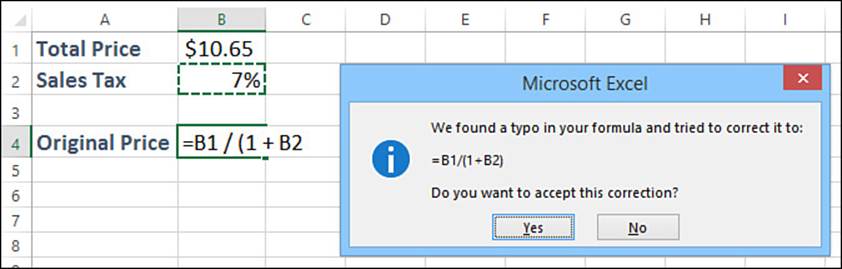
Figure 5.1 If you miss a parenthesis, Excel attempts to fix the problem and displays this dialog box to ask if you want to accept the correction.
Caution
Excel doesn’t always fix missing parentheses correctly. It tends to add the missing parenthesis to the end of the formula, which is often not what you want. Therefore, always check Excel’s proposed solution carefully before accepting it.
To help you avoid missing or mismatched parentheses, Excel provides two visual clues in the formula itself when you’re editing it:
![]() The first clue occurs when you type a right parenthesis. Excel highlights both the right parenthesis and its corresponding left parenthesis. If you type what you think is the last right parenthesis and Excel doesn’t highlight the first left parenthesis, your parentheses are unbalanced.
The first clue occurs when you type a right parenthesis. Excel highlights both the right parenthesis and its corresponding left parenthesis. If you type what you think is the last right parenthesis and Excel doesn’t highlight the first left parenthesis, your parentheses are unbalanced.
![]() The second clue occurs when you use the left and right arrow keys to navigate a formula. When you cross over a parenthesis, Excel highlights the other parenthesis in the pair and formats both parentheses with the same color.
The second clue occurs when you use the left and right arrow keys to navigate a formula. When you cross over a parenthesis, Excel highlights the other parenthesis in the pair and formats both parentheses with the same color.
Erroneous Formula Results
If a formula produces no warnings or error values, the result might still be in error. If the result of a formula is incorrect, here are a few techniques that can help you understand and fix the problem:
![]() Calculate complex formulas one term at a time. In the formula bar, select the expression you want to calculate and then press F9. Excel converts the expression into its value. Make sure that you press the Esc key when you’re done to avoid entering the formula with just the calculated values.
Calculate complex formulas one term at a time. In the formula bar, select the expression you want to calculate and then press F9. Excel converts the expression into its value. Make sure that you press the Esc key when you’re done to avoid entering the formula with just the calculated values.
![]() Evaluate the formula. You can step through the various parts of a formula.
Evaluate the formula. You can step through the various parts of a formula.
![]() To learn how to evaluate formulas, see “Evaluating Formulas,” p. 126.
To learn how to evaluate formulas, see “Evaluating Formulas,” p. 126.
![]() Break up long or complex formulas. One of the most problematic aspects of formula troubleshooting is making sense out of long formulas. The previous techniques can help (by enabling you to evaluate parts of the formula), but it’s usually best to keep your formulas as short as you can at first. When you get things working properly, you often can combine formulas for a more efficient model.
Break up long or complex formulas. One of the most problematic aspects of formula troubleshooting is making sense out of long formulas. The previous techniques can help (by enabling you to evaluate parts of the formula), but it’s usually best to keep your formulas as short as you can at first. When you get things working properly, you often can combine formulas for a more efficient model.
![]() Recalculate all formulas. A particular formula might display the wrong result because other formulas on which it depends need to be recalculated. This is particularly true if one or more of those formulas use custom VBA functions. Press Ctrl+Alt+F9 to recalculate all worksheet formulas.
Recalculate all formulas. A particular formula might display the wrong result because other formulas on which it depends need to be recalculated. This is particularly true if one or more of those formulas use custom VBA functions. Press Ctrl+Alt+F9 to recalculate all worksheet formulas.
![]() Pay attention to operator precedence. As explained in Chapter 3, Excel’s operator precedence means that certain operations are performed before others. An erroneous formula result could therefore be caused by Excel’s precedence order. To control precedence, use parentheses.
Pay attention to operator precedence. As explained in Chapter 3, Excel’s operator precedence means that certain operations are performed before others. An erroneous formula result could therefore be caused by Excel’s precedence order. To control precedence, use parentheses.
![]() Watch out for nonblank “blank” cells. A cell might appear to be blank but actually contain data or even a formula. For example, some users “clear” a cell by pressing the spacebar, and Excel then treats the cell as nonblank. Similarly, some formulas return an empty string instead of a value. (For example, see the IF() function formula earlier in this chapter for avoiding the #DIV/0! error.)
Watch out for nonblank “blank” cells. A cell might appear to be blank but actually contain data or even a formula. For example, some users “clear” a cell by pressing the spacebar, and Excel then treats the cell as nonblank. Similarly, some formulas return an empty string instead of a value. (For example, see the IF() function formula earlier in this chapter for avoiding the #DIV/0! error.)
![]() Watch unseen values. In a large model, your formula could be using cells that you can’t see because they’re offscreen or on another sheet. Excel’s Watch Window enables you to keep an eye on the current value of one or more cells.
Watch unseen values. In a large model, your formula could be using cells that you can’t see because they’re offscreen or on another sheet. Excel’s Watch Window enables you to keep an eye on the current value of one or more cells.
![]() To learn about the Watch Window, see “Watching Cell Values,” p. 126.
To learn about the Watch Window, see “Watching Cell Values,” p. 126.
Fixing Circular References
A circular reference occurs when a formula refers to its own cell. This can happen in one of two ways:
![]() Directly—The formula explicitly references its own cell. For example, a circular reference would result if the following formula were entered into cell A1:
Directly—The formula explicitly references its own cell. For example, a circular reference would result if the following formula were entered into cell A1:
=A1+A2
![]() Indirectly—The formula references a cell or function that, in turn, references the formula’s cell. For example, suppose that cell A1 contains the following formula:
Indirectly—The formula references a cell or function that, in turn, references the formula’s cell. For example, suppose that cell A1 contains the following formula:
=A5*10
![]() A circular reference would result if cell A5 referred to cell A1, as in this example:
A circular reference would result if cell A5 referred to cell A1, as in this example:
=SUM(A1:D1)
When Excel detects a circular reference, it displays the dialog box shown in Figure 5.2.
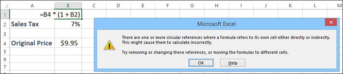
Figure 5.2 If you attempt to enter a formula that contains a circular reference, Excel displays this dialog box.
When you click OK, Excel displays tracer arrows that connect the cells involved in the circular reference. (Tracers are discussed in detail later in this chapter; see “Auditing a Worksheet.”) Knowing which cells are involved enables you to correct the formula in one of them to solve the problem.
Handling Formula Errors with IFERROR()
Earlier you saw how to use the IF() function to avoid a #DIV/0! error by testing the value of the formula divisor to see if it equals 0. This works fine if you can anticipate the specific type of error the user may make. However, in many instances you can’t know the exact nature of the error in advance. For example, the simple formula =GrossProfit/Sales would generate a #DIV/0! error if Sales equals 0. However, it would generate a #NAME? error if the name GrossProfit or the name Sales no longer exists, or it would generate a #REF! error if the cells associated with one or both of GrossProfit and Sales were deleted.
If you want to handle errors gracefully in your worksheets, it’s often best to assume that any error can occur. Fortunately, that doesn’t mean you have to construct complex tests using deeply nested IF() functions that check for every error type (#DIV/0!, #N/A, and so on). Instead, Excel enables you to use a simple test for any error.
In legacy versions of Excel, you’d use the ISERROR(value) function, where value is an expression. Here’s what it does: If value generates any error, ISERROR() returns True; if value doesn’t generate an error, ISERROR() returns False. You would then incorporate this into anIF() test, using the following general syntax:
=IF(ISERROR(expression), ErrorResult, expression)
If expression generates an error, this formula returns the ErrorResult value (such as the null string or an error message); otherwise, it returns the result of expression. Here’s an example that uses the GrossProfit / Sales expression:
=IF(ISERROR(GrossProfit / Sales), "", GrossProfit / Sales)
The problem with using IF() and ISERROR() to handle errors is that you must input the expression twice: once in the ISERROR() function and again as the False result in the IF() function. This not only takes longer to input but also makes your formulas harder to maintain because if you make changes to the expression, you have to change both instances.
Excel makes handling formula errors much easier by offering the IFERROR() function, which essentially combines IF() and ISERROR() into a single function:
IFERROR(value, value_if_error)

If the value expression doesn’t generate an error, IFERROR() returns the expression result; otherwise, it returns value_if_error (which might be the null string or an error message). Here’s an example:
=IFERROR((GrossProfit / Sales), "")
As you can see, this is much better than using IF() and ISERROR(). It’s shorter, easier to read, and easier to maintain because you use your expression only once.
Note
If you want to handle the specific case of the #N/A error, use the IFNA(value, value_if_na) function. Here, value is the expression that you’re testing for the #N/A error, and value_if_na is the value to return if value returns the #N/A error.
Using the Formula Error Checker
If you use Microsoft Word, you’re probably familiar with the wavy green lines that appear under words and phrases that the grammar checker has flagged as being incorrect. The grammar checker operates by using a set of rules that determine correct grammar and syntax. As you type, the grammar checker operates in the background, constantly monitoring your writing. If something you write goes against one of the grammar checker’s rules, the wavy line appears to let you know there’s a problem.
Excel has a similar feature: the formula error checker. Like the grammar checker, the formula error checker uses a set of rules to determine correctness, and it operates in the background to monitor your formulas. If it detects something amiss, it displays an error indicator—a green triangle—in the upper-left corner of the cell containing the formula, as shown in Figure 5.3.
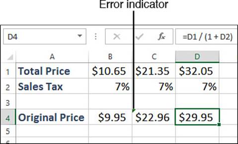
Figure 5.3 If Excel’s formula error checker detects a problem, it displays a green triangle in the upper-left corner of the formula’s cell.
Choosing an Error Action
When you select the cell with the formula error, Excel displays a formula error icon beside the cell. If you hover your mouse pointer over the icon, a pop-up message describes the error, as shown in Figure 5.4. The formula error icon drop-down list contains the following actions:
![]() Corrective action—This is a command (the name of which depends on the type of error) that Excel believes either will fix the problem or help you troubleshoot the error. In Figure 5.4, for example, Excel is reporting that the formula in cell C3 differs from its neighboring formulas. (In the formula bar, the expression in the parentheses should be 1+C2 instead of 1-C2.) In this case, the corrective action command in the formula error icon is Copy Formula from Left. Or, if Excel can’t suggest a solution, it might show the command Show Calculation Steps, which runs the Evaluate Formula feature. See “Evaluating Formulas,” later in this chapter.
Corrective action—This is a command (the name of which depends on the type of error) that Excel believes either will fix the problem or help you troubleshoot the error. In Figure 5.4, for example, Excel is reporting that the formula in cell C3 differs from its neighboring formulas. (In the formula bar, the expression in the parentheses should be 1+C2 instead of 1-C2.) In this case, the corrective action command in the formula error icon is Copy Formula from Left. Or, if Excel can’t suggest a solution, it might show the command Show Calculation Steps, which runs the Evaluate Formula feature. See “Evaluating Formulas,” later in this chapter.
![]() Help on This Error—Select this option to get information on the error via the Excel Help system.
Help on This Error—Select this option to get information on the error via the Excel Help system.
![]() Ignore Error—Select this option to leave the formula as is.
Ignore Error—Select this option to leave the formula as is.
![]() Edit in Formula Bar—Select this option to display the formula in Edit mode in the formula bar. You can then fix the problem by editing the formula.
Edit in Formula Bar—Select this option to display the formula in Edit mode in the formula bar. You can then fix the problem by editing the formula.
![]() Error-Checking Options—Select this option to display the Formulas tab of the Excel Options dialog box (discussed next).
Error-Checking Options—Select this option to display the Formulas tab of the Excel Options dialog box (discussed next).
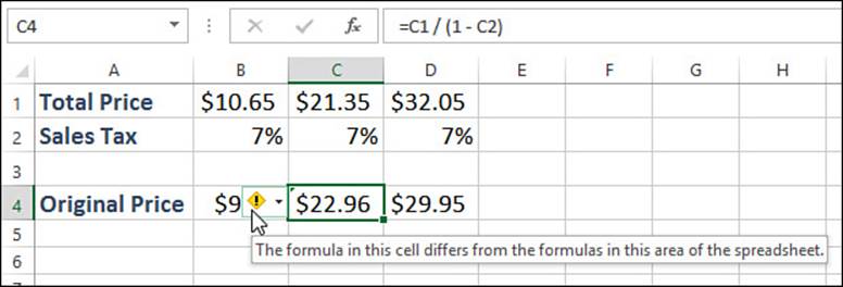
Figure 5.4 Select the cell containing the error and then move the mouse pointer over the formula error icon to see a description of the error.
Setting Error Checker Options
Like Word’s grammar checker, Excel’s formula error checker has a number of options that control how it works and which errors it flags. To see these options, you have two choices:
![]() Select File, Options to display the Excel Options dialog box and then click Formulas.
Select File, Options to display the Excel Options dialog box and then click Formulas.
![]() Select Error-Checking Options in the formula error icon’s drop-down list (as described in the previous section).
Select Error-Checking Options in the formula error icon’s drop-down list (as described in the previous section).
Either way, the options appear in the Error Checking and Error Checking Rules sections in the Formulas tab, as shown in Figure 5.5.
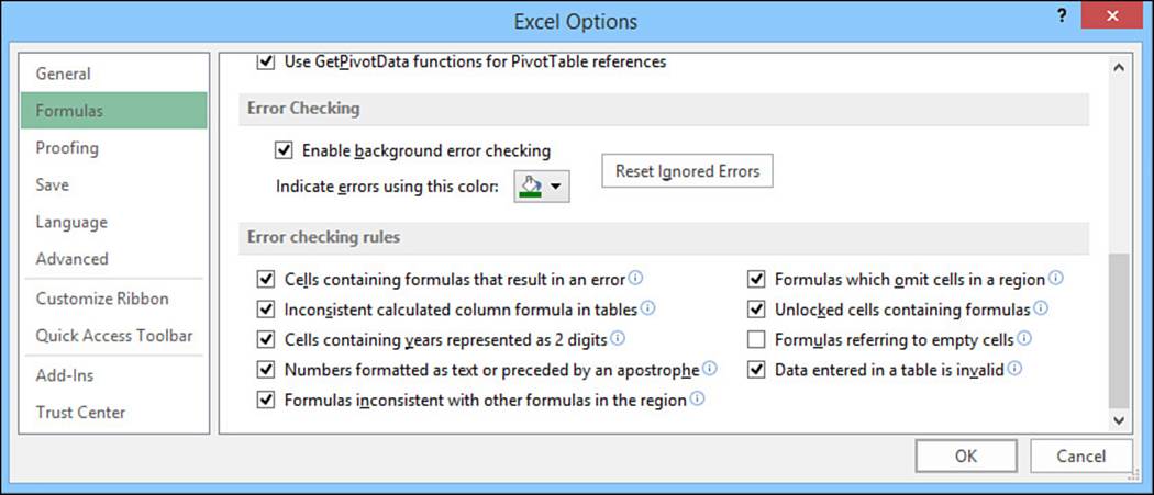
Figure 5.5 In the Formulas tab, the Error Checking and Error Checking Rules sections contain the options that govern the workings of the formula error checker.
Here’s a rundown of the available options:
![]() Enable Background Error Checking—This check box toggles the formula error checker’s background operation on and off. If you turn off the background checking, you can run a check at any time by choosing Formulas, Error Checking.
Enable Background Error Checking—This check box toggles the formula error checker’s background operation on and off. If you turn off the background checking, you can run a check at any time by choosing Formulas, Error Checking.
![]() Indicate Errors Using This Color—Use this color palette to click the color of the error indicator.
Indicate Errors Using This Color—Use this color palette to click the color of the error indicator.
![]() Reset Ignored Errors—If you’ve ignored one or more errors, you can redisplay the error indicators by clicking this button.
Reset Ignored Errors—If you’ve ignored one or more errors, you can redisplay the error indicators by clicking this button.
![]() Cells Containing Formulas That Result in an Error—When this check box is selected, the formula error checker flags formulas that evaluate to #DIV/0!, #NAME?, or any of the other error values discussed earlier.
Cells Containing Formulas That Result in an Error—When this check box is selected, the formula error checker flags formulas that evaluate to #DIV/0!, #NAME?, or any of the other error values discussed earlier.
![]() Inconsistent Calculated Column Formula in Tables—When this check box is selected, Excel examines the formulas in a table’s calculated column and flags any cell that contains a formula with a different structure than the other cells in the column. The formula error icon for this error includes the command Restore to Calculated Column Formula, which enables you to update the formula so that it’s consistent with the rest of the column.
Inconsistent Calculated Column Formula in Tables—When this check box is selected, Excel examines the formulas in a table’s calculated column and flags any cell that contains a formula with a different structure than the other cells in the column. The formula error icon for this error includes the command Restore to Calculated Column Formula, which enables you to update the formula so that it’s consistent with the rest of the column.
![]() Cells Containing Years Represented as 2 Digits—When this check box is selected, the formula error checker flags formulas that contain date text strings in which the year contains only two digits (a possibly ambiguous situation because the string could refer to a date in either the 1900s or the 2000s). In such a case, the list of options supplied in the formula error icon contains two commands—Convert XX to 19XX and Convert XX to 20XX—that enable you to convert the two-digit year to a four-digit year.
Cells Containing Years Represented as 2 Digits—When this check box is selected, the formula error checker flags formulas that contain date text strings in which the year contains only two digits (a possibly ambiguous situation because the string could refer to a date in either the 1900s or the 2000s). In such a case, the list of options supplied in the formula error icon contains two commands—Convert XX to 19XX and Convert XX to 20XX—that enable you to convert the two-digit year to a four-digit year.
![]() Numbers Formatted as Text or Preceded by an Apostrophe—When this check box is selected, the formula error checker flags cells that contain a number that is either formatted as text or preceded by an apostrophe. In such a case, the list of options supplied in the formula error icon contains the Convert to Number command to convert the text to its numeric equivalent.
Numbers Formatted as Text or Preceded by an Apostrophe—When this check box is selected, the formula error checker flags cells that contain a number that is either formatted as text or preceded by an apostrophe. In such a case, the list of options supplied in the formula error icon contains the Convert to Number command to convert the text to its numeric equivalent.
![]() Formulas Inconsistent with Other Formulas in the Region—When this check box is selected, the formula error checker flags formulas that are structured differently from similar formulas in the surrounding area. In such a case, the list of options supplied in the formula error icon contains a command such as Copy Formula from Left to bring the formula into consistency with the surrounding cells.
Formulas Inconsistent with Other Formulas in the Region—When this check box is selected, the formula error checker flags formulas that are structured differently from similar formulas in the surrounding area. In such a case, the list of options supplied in the formula error icon contains a command such as Copy Formula from Left to bring the formula into consistency with the surrounding cells.
![]() Formulas Which Omit Cells in a Region—When this check box is selected, the formula error checker flags formulas that omit cells that are adjacent to a range referenced in the formula. For example, suppose that the formula is =AVERAGE(C4:C21), where C4:C21 is a range of numeric values. If cell C3 also contains a numeric value, the formula error checker flags the formula to alert you to the possibility that you missed including cell C3 in the formula. Figure 5.6 shows this example. In such a case, the list of options supplied in the formula error icon will contain the command Update Formula to Include Cells to adjust the formula automatically.
Formulas Which Omit Cells in a Region—When this check box is selected, the formula error checker flags formulas that omit cells that are adjacent to a range referenced in the formula. For example, suppose that the formula is =AVERAGE(C4:C21), where C4:C21 is a range of numeric values. If cell C3 also contains a numeric value, the formula error checker flags the formula to alert you to the possibility that you missed including cell C3 in the formula. Figure 5.6 shows this example. In such a case, the list of options supplied in the formula error icon will contain the command Update Formula to Include Cells to adjust the formula automatically.
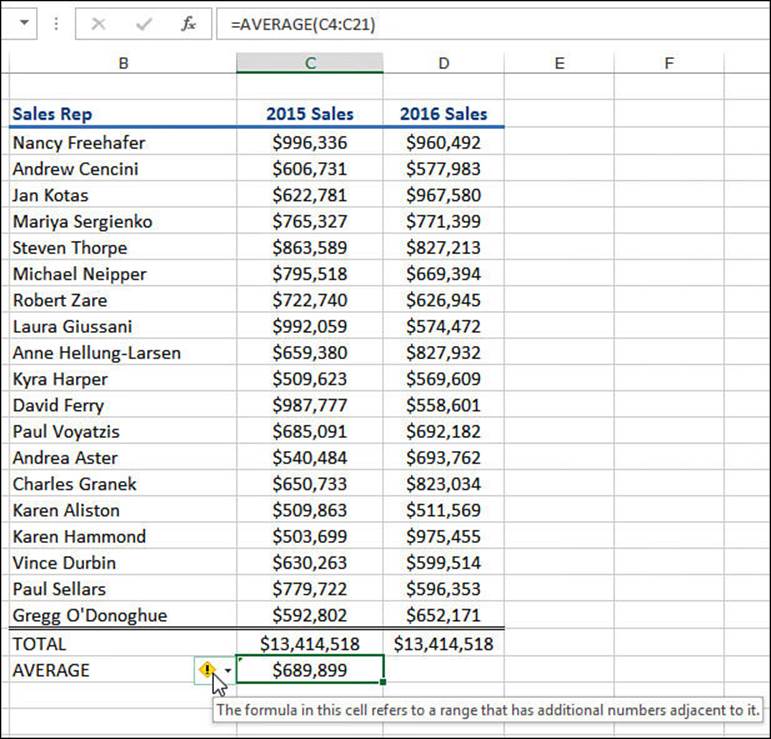
Figure 5.6 The formula error checker can flag formulas that omit cells that are adjacent to a range referenced by the formula. In this case, the formula in C23 should include cell C3.
![]() Unlocked Cells Containing Formulas—When this check box is selected, the formula error checker flags formulas that reside in unlocked cells. This isn’t an error so much as a warning that other people could tamper with the formula even after you have protected the sheet. In such a case, the list of options supplied in the formula error icon will contain the command Lock Cell to lock the cell and prevent users from changing the formula after you protect the sheet.
Unlocked Cells Containing Formulas—When this check box is selected, the formula error checker flags formulas that reside in unlocked cells. This isn’t an error so much as a warning that other people could tamper with the formula even after you have protected the sheet. In such a case, the list of options supplied in the formula error icon will contain the command Lock Cell to lock the cell and prevent users from changing the formula after you protect the sheet.
![]() Formulas Referring to Empty Cells—When this check box is selected, the formula error checker flags formulas that reference empty cells. In such a case, the list of options supplied in the formula error icon will contain the command Trace Empty Cell to enable you to find the empty cell. (At this point, you can either enter data into the cell or adjust the formula so that it doesn’t reference the cell.)
Formulas Referring to Empty Cells—When this check box is selected, the formula error checker flags formulas that reference empty cells. In such a case, the list of options supplied in the formula error icon will contain the command Trace Empty Cell to enable you to find the empty cell. (At this point, you can either enter data into the cell or adjust the formula so that it doesn’t reference the cell.)
![]() Data Entered in a Table Is Invalid—When this check box is selected, the formula error checker flags cells that violate a table’s data-validation rules. This can happen if you set up a data-validation rule with only a Warning or Information style, in which case the user can still opt to enter the invalid data. In such cases, the formula error checker will flag the cells that contain invalid data. The formula error icon list includes the Display Type Information command, which shows the data-validation rule that the cell data violates.
Data Entered in a Table Is Invalid—When this check box is selected, the formula error checker flags cells that violate a table’s data-validation rules. This can happen if you set up a data-validation rule with only a Warning or Information style, in which case the user can still opt to enter the invalid data. In such cases, the formula error checker will flag the cells that contain invalid data. The formula error icon list includes the Display Type Information command, which shows the data-validation rule that the cell data violates.
![]() For a detailed look at data validation, see “Applying Data-Validation Rules to Cells,” p. 100.
For a detailed look at data validation, see “Applying Data-Validation Rules to Cells,” p. 100.
Auditing a Worksheet
As you’ve seen, some formula errors result from referencing other cells that contain errors or inappropriate values. The first step in troubleshooting these kinds of formula problems is to determine which cell (or group of cells) is causing an error. This is straightforward if the formula references only a single cell, but it gets progressively more difficult as the number of references increases. (Another complicating factor is the use of range names because it won’t be obvious which range each name is referencing.)
To determine which cells are wreaking havoc on your formulas, you can use Excel’s auditing features to visualize and trace a formula’s input values and error sources.
Understanding Auditing
Excel’s formula-auditing features operate by creating tracers—arrows that literally point out the cells involved in a formula. You can use tracers to find three kinds of cells:
![]() Precedents—These are cells that are directly or indirectly referenced in a formula. For example, suppose that cell B4 contains the formula =B2; then B2 is a direct precedent of B4. Now suppose that cell B2 contains the formula =A2/2; this makes A2 a direct precedent of B2, but it’s also an indirect precedent of cell B4.
Precedents—These are cells that are directly or indirectly referenced in a formula. For example, suppose that cell B4 contains the formula =B2; then B2 is a direct precedent of B4. Now suppose that cell B2 contains the formula =A2/2; this makes A2 a direct precedent of B2, but it’s also an indirect precedent of cell B4.
![]() Dependents—These are cells that are directly or indirectly referenced by a formula in another cell. In the preceding example, cell B2 is a direct dependent of A2, and B4 is an indirect dependent of A2.
Dependents—These are cells that are directly or indirectly referenced by a formula in another cell. In the preceding example, cell B2 is a direct dependent of A2, and B4 is an indirect dependent of A2.
![]() Errors—These are cells that contain an error value and are directly or indirectly referenced in a formula (and therefore cause the same error to appear in the formula).
Errors—These are cells that contain an error value and are directly or indirectly referenced in a formula (and therefore cause the same error to appear in the formula).
Figure 5.7 shows a worksheet with three examples of tracer arrows:
![]() Cell B4 contains the formula =B2, and B2 contains =A2/2. The arrows (they’re blue onscreen) point out the precedents (direct and indirect) of B4.
Cell B4 contains the formula =B2, and B2 contains =A2/2. The arrows (they’re blue onscreen) point out the precedents (direct and indirect) of B4.
![]() Cell D4 contains the formula =D2, and D2 contains =D1/0. The latter produces the #DIV/0! error. Therefore, the same error appears in cell D4. The arrow (it’s red onscreen) is pointing out the source of the error.
Cell D4 contains the formula =D2, and D2 contains =D1/0. The latter produces the #DIV/0! error. Therefore, the same error appears in cell D4. The arrow (it’s red onscreen) is pointing out the source of the error.
![]() Cell G4 contains the formula =Sheet2!A1. Excel displays the dashed arrow with the worksheet icon whenever the precedent or dependent exists on a different worksheet.
Cell G4 contains the formula =Sheet2!A1. Excel displays the dashed arrow with the worksheet icon whenever the precedent or dependent exists on a different worksheet.
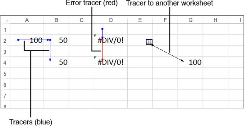
Figure 5.7 The three types of tracer arrows.
Note
You can download this chapter’s sample workbook at www.mcfedries.com/books/book.php?title=excel-2016-formulas-and-functions.
Tracing Cell Precedents
To trace cell precedents, follow these steps:
1. Select the cell that contains the formula whose precedents you want to trace.
2. Select Formulas, Trace Precedents. Excel adds a tracer arrow to each direct precedent.
3. Keep repeating step 2 to see more levels of precedents.
Tip
You also can trace precedents by double-clicking the cell, provided that you turn off in-cell editing. You do this by choosing File, Options to display the Excel Options dialog box, clicking Advanced, and then deselecting the Allow Editing Directly in Cells check box. Now when you double-click a cell, Excel selects the formula’s precedents.
Tracing Cell Dependents
Here are the steps to follow to trace cell dependents:
1. Select the cell whose dependents you want to trace.
2. Select Formulas, Trace Dependents. Excel adds a tracer arrow to each direct dependent.
3. Keep repeating step 2 to see more levels of dependents.
Tracing Cell Errors
To trace cell errors, follow these steps:
1. Select the cell that contains the error you want to trace.
2. Select Formulas, Error Checking, Trace Error. Excel adds a tracer arrow to each cell that produced the error.
Removing Tracer Arrows
To remove the tracer arrows, you have three choices:
![]() To remove all the tracer arrows, select Formulas, Remove Arrows.
To remove all the tracer arrows, select Formulas, Remove Arrows.
![]() To remove precedent arrows one level at a time, select Formulas, drop down the Remove Arrows list, and select Remove Precedent Arrows.
To remove precedent arrows one level at a time, select Formulas, drop down the Remove Arrows list, and select Remove Precedent Arrows.
![]() To remove dependent arrows one level at a time, select Formulas, drop down the Remove Arrows list, and select Remove Dependent Arrows.
To remove dependent arrows one level at a time, select Formulas, drop down the Remove Arrows list, and select Remove Dependent Arrows.
Evaluating Formulas
Earlier, you learned that you can troubleshoot a wonky formula by evaluating parts of it. You do this by selecting the part of the formula you want to evaluate and then pressing F9. This works fine, but it can be tedious in a long or complex formula, and there’s always a danger that you might accidentally confirm a partially evaluated formula and lose your work.
A better solution is to use Excel’s Evaluate Formula feature. It does the same thing as the F9 technique, but it’s easier and safer. Here’s how it works:
1. Select the cell that contains the formula you want to evaluate.
2. Select Formulas, Evaluate Formula. Excel displays the Evaluate Formula dialog box.
3. The current term in the formula is underlined in the Evaluation box. At each step, you select from one or more of the following buttons:
• Evaluate—Click this button to display the current value of the underlined term.
• Step In—Click this button to display the first dependent of the underlined term. If that dependent also has a dependent, click this button again to see it (see Figure 5.8).
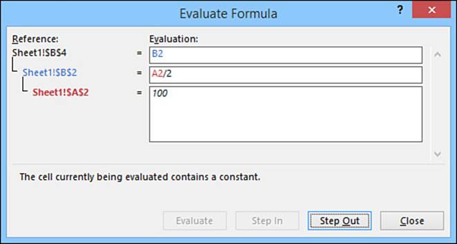
Figure 5.8 With the Evaluate Formula feature, you can “step into” the formula to display its dependent cells.
• Step Out—Click this button to hide a dependent and evaluate its precedent.
4. Repeat step 3 until you’ve completed your evaluation.
5. Click Close.
Watching Cell Values
In the precedent tracer example shown in Figure 5.7, the formula in cell G4 refers to a cell in another worksheet, which is represented in the trace by a worksheet icon. In other words, you can’t see the formula cell and the precedent cell at the same time. This could also happen if the precedent existed on another workbook or even elsewhere on the same sheet if you’re working with a large model.
This is a problem because there’s no easy way to determine the current contents or value of the unseen precedent. If you’re having a problem, troubleshooting requires that you track down the far-off precedent to see if it might be the culprit. That’s bad enough with a single unseen cell, but what if your formula refers to 5 or 10 such cells? And what if those cells are scattered in different worksheets and workbooks?
This level of hassle—not at all uncommon in the spreadsheet world—was no doubt the inspiration behind an elegant solution: the Watch Window. This window enables you to keep tabs on both the value and the formula in any cell in any worksheet in any open workbook. Here’s how you set up a watch:
1. Switch to the workbook that contains the cell or cells you want to watch.
2. Select Formulas, Watch Window. Excel displays the Watch Window.
3. Click Add Watch. Excel displays the Add Watch dialog box.
4. Either select the cell you want to watch or type in a reference formula for the cell (for example, =A1). Note that you can select a range to add multiple cells to the Watch Window.
5. Click Add. Excel adds the cell or cells to the Watch Window, as shown in Figure 5.9.
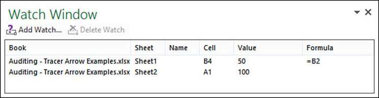
Figure 5.9 Use the Watch Window to keep an eye on the values and formulas of unseen cells that reside in other worksheets or workbooks.
When you no longer need a watch, you should remove it to avoid cluttering the Watch Window. To remove a watch, select Formulas, Watch Window to open the Watch Window, click the watch, and then click Delete Watch.
From Here
![]() To learn how to paste range names, see “Pasting a List of Range Names in a Worksheet,” p. 48.
To learn how to paste range names, see “Pasting a List of Range Names in a Worksheet,” p. 48.
![]() For the details of Excel’s operator precedence rules, see “Understanding Operator Precedence,” p. 57.
For the details of Excel’s operator precedence rules, see “Understanding Operator Precedence,” p. 57.
![]() To learn more about iteration, see “Using Iteration and Circular References,” p. 93.
To learn more about iteration, see “Using Iteration and Circular References,” p. 93.
![]() For a detailed look at data validation, see “Applying Data-Validation Rules to Cells,” p. 100.
For a detailed look at data validation, see “Applying Data-Validation Rules to Cells,” p. 100.
![]() To learn about the IF() worksheet function, see “Using the IF() Function,” p. 164.
To learn about the IF() worksheet function, see “Using the IF() Function,” p. 164.
![]() For the details of Excel’s table features, see Chapter 13, “Analyzing Data with Tables,” p. 291.
For the details of Excel’s table features, see Chapter 13, “Analyzing Data with Tables,” p. 291.
All materials on the site are licensed Creative Commons Attribution-Sharealike 3.0 Unported CC BY-SA 3.0 & GNU Free Documentation License (GFDL)
If you are the copyright holder of any material contained on our site and intend to remove it, please contact our site administrator for approval.
© 2016-2026 All site design rights belong to S.Y.A.