Excel® 2016 Formulas and Functions (2016)
Part II: Harnessing the Power of Functions
6. Understanding Functions
In This Chapter
About Excel’s Functions
The Structure of a Function
Typing a Function into a Formula
Using the Insert Function Feature
Loading the Analysis ToolPak
The formulas that you can construct based on the information presented in Part I, “Mastering Excel Ranges and Formulas,” can range from simple additions and subtractions to powerful iteration-based solutions for otherwise difficult problems. Formulas that combine Excel’s operators with basic operands such as numeric and string values are the bread and butter of any spreadsheet.
But to get to the real meat of a spreadsheet model, you need to expand your formula repertoire to include Excel’s worksheet functions. Dozens of these functions exist, and they’re essential to making your worksheet easier to work with and more powerful. Excel has various function categories, including the following:
![]() Text
Text
![]() Logical
Logical
![]() Information
Information
![]() Lookup and reference
Lookup and reference
![]() Date and time
Date and time
![]() Math and trigonometry
Math and trigonometry
![]() Statistical
Statistical
![]() Financial
Financial
![]() Database and table
Database and table
This chapter gives you a short introduction to Excel’s built-in worksheet functions. You’ll find out what the functions are, what they can do, and how to use them. The next six chapters give you detailed descriptions of the functions in the preceding list of categories. (The exceptions are the database and table category, which I cover in Chapter 13, “Analyzing Data with Tables,” and the financial category, which I cover in Part IV, “Building Financial Formulas.”)
Note
You can even create your own custom functions when Excel’s built-in functions aren’t up to the task you need to complete. You build these functions by using the Visual Basic for Applications (VBA) macro language, and it’s easier than you think. See the book Excel 2016 VBA and Macros (Que, 2016).
About Excel’s Functions
Functions are formulas that Excel has predefined. They’re designed to take you beyond the basic arithmetic and text formulas you’ve seen so far. They do this in three ways:
![]() Functions make simple but cumbersome formulas easier to use. For example, suppose that you want to add a list of 100 numbers in a column, starting at cell A1 and finishing at cell A100. It’s unlikely that you have the time or patience to enter 100 separate additions in a cell (that is, the formula =A1+A2+...+A100). Luckily, there’s an alternative: the SUM() function. With this function, you would simply enter =SUM(A1:A100).
Functions make simple but cumbersome formulas easier to use. For example, suppose that you want to add a list of 100 numbers in a column, starting at cell A1 and finishing at cell A100. It’s unlikely that you have the time or patience to enter 100 separate additions in a cell (that is, the formula =A1+A2+...+A100). Luckily, there’s an alternative: the SUM() function. With this function, you would simply enter =SUM(A1:A100).
![]() Functions enable you to include in your worksheets complex mathematical expressions that otherwise would be difficult or impossible to construct using simple arithmetic operators. For example, determining a mortgage payment given the principal, interest, and term is a complicated matter at best, but you can do it with Excel’s PMT() function just by entering a few arguments.
Functions enable you to include in your worksheets complex mathematical expressions that otherwise would be difficult or impossible to construct using simple arithmetic operators. For example, determining a mortgage payment given the principal, interest, and term is a complicated matter at best, but you can do it with Excel’s PMT() function just by entering a few arguments.
![]() Functions enable you to include data in your applications that you couldn’t access otherwise. For example, the INFO() function can tell you how much memory is available on your system, what operating system you’re using, what version number it is, and more. Similarly, the powerful IF() function enables you to test the contents of a cell—for example, to see whether it contains a particular value or an error—and then perform an action accordingly, depending on the result.
Functions enable you to include data in your applications that you couldn’t access otherwise. For example, the INFO() function can tell you how much memory is available on your system, what operating system you’re using, what version number it is, and more. Similarly, the powerful IF() function enables you to test the contents of a cell—for example, to see whether it contains a particular value or an error—and then perform an action accordingly, depending on the result.
As you can see, functions are a powerful addition to your worksheet-building arsenal. With proper use of these tools, there is no practical limit to the kinds of models you can create.
The Structure of a Function
Every function has the same basic form:
FUNCTION(argument1, argument2, ...)
The FUNCTION part is the name of the function, which always appears in uppercase letters (such as SUM or PMT). Note, however, that you don’t need to type in the function name using uppercase letters. Whatever case you use, Excel automatically converts the name to all uppercase. In fact, it’s good practice to enter function names using only lowercase letters. That way, if Excel doesn’t convert the function name to uppercase, you know that it doesn’t recognize the name, which means you probably misspelled it.
The items that appear within the parentheses and separated by commas are the function arguments. The arguments are the function’s inputs—the data the function uses to perform its calculations. With respect to arguments, functions come in two flavors:
![]() No arguments—Many functions don’t require any arguments. For example, the NOW() function returns the current date and time, and it doesn’t require arguments.
No arguments—Many functions don’t require any arguments. For example, the NOW() function returns the current date and time, and it doesn’t require arguments.
![]() One or more arguments—Most functions accept at least one argument, and some accept as many as nine or ten arguments. These arguments fall into two categories: required and optional. Required arguments are the arguments you must include when you use the function; otherwise, the formula will generate an error. You use the optional arguments only if your formula needs them.
One or more arguments—Most functions accept at least one argument, and some accept as many as nine or ten arguments. These arguments fall into two categories: required and optional. Required arguments are the arguments you must include when you use the function; otherwise, the formula will generate an error. You use the optional arguments only if your formula needs them.
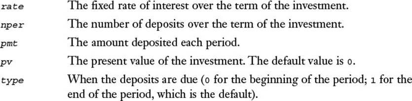
Let’s look at an example. The FV() function determines the future value of a regular investment, based on three required arguments and two optional ones:
FV(rate, nper, pmt[, pv][, type])
This is called the function syntax. Three conventions are at work here and throughout the rest of this book:
![]() Italic type indicates a placeholder. That is, when you use the function, you replace the placeholder with an actual value.
Italic type indicates a placeholder. That is, when you use the function, you replace the placeholder with an actual value.
![]() Arguments surrounded by square brackets are optional.
Arguments surrounded by square brackets are optional.
![]() All other arguments are required.
All other arguments are required.
Caution
Be careful how you use commas in functions that have optional arguments. If you omit the last optional argument, you must leave out the comma that precedes the argument. For example, if you omit just the type argument from FV(), you write the function like so:
FV(rate, nper, pmt, pv)
However, if you omit an optional argument within the syntax, you need to include all the commas so that there is no ambiguity about which value refers to which argument. For example, if you omit the pv argument from FV(), you write the function like this:
FV(rate, nper, pmt, , type)
For each argument placeholder, you substitute an appropriate value. For example, in the FV() function, you substitute rate with a decimal value between 0 and 1, nper with an integer, and pmt with a dollar amount. Arguments can take any of the following forms:
![]() Literal alphanumeric values
Literal alphanumeric values
![]() Expressions
Expressions
![]() Cell or range references
Cell or range references
![]() Range names
Range names
![]() Arrays
Arrays
![]() The result of another function
The result of another function
The function operates by processing the inputs and then returning a result. For example, the FV() function returns the total value of the investment at the end of the term. Figure 6.1 shows a simple future-value calculator that uses this function. (In case you’re wondering, I entered the Payment value in cell B4 as negative because Excel always treats any money you have to pay as a negative number.)
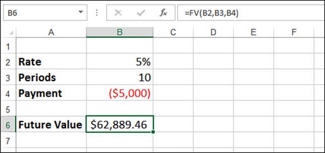
Figure 6.1 This example of the FV() function uses the values in cells B2, B3, and B4 as inputs for calculating the future value of an investment.
Note
You can download this chapter’s sample workbook at www.mcfedries.com/books/book.php?title=excel-2016-formulas-and-functions.
Typing a Function into a Formula
You always use a function as part of a cell formula. So, even if you’re using the function by itself, you still need to precede it with an equal sign. Whether you use a function on its own or as part of a larger formula, here are a few rules and guidelines to follow:
![]() You can enter the function name in either uppercase or lowercase letters. Excel always converts function names to uppercase.
You can enter the function name in either uppercase or lowercase letters. Excel always converts function names to uppercase.
![]() Always enclose function arguments in parentheses.
Always enclose function arguments in parentheses.
![]() Always separate multiple arguments with commas. (You might want to add a space after each comma to make a function more readable. Excel ignores the extra spaces.)
Always separate multiple arguments with commas. (You might want to add a space after each comma to make a function more readable. Excel ignores the extra spaces.)
![]() You can use a function as an argument for another function. This is called nesting functions. For example, the function AVERAGE(SUM(A1:A10), SUM(B1:B15)) sums two columns of numbers and returns the average of the two sums.
You can use a function as an argument for another function. This is called nesting functions. For example, the function AVERAGE(SUM(A1:A10), SUM(B1:B15)) sums two columns of numbers and returns the average of the two sums.
In Chapter 2, “Using Range Names,” I introduced you to Excel’s AutoComplete feature for range names that shows you a list of named ranges that begin with the characters you’ve typed in a formula. That feature also applies to functions. As you can see in Figure 6.2, when you begin typing a name in Excel, the program displays a list of the functions that start with the letters you’ve typed and displays a description of the currently selected function. Select the function you want to use and then press Tab to include it in the formula (or double-click the function).
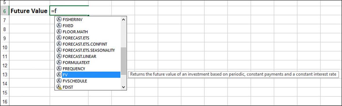
Figure 6.2 When you begin typing a name in Excel, the program displays a list of functions with names that begin with the typed characters.
![]() For the details on AutoComplete for named ranges, see “Working with AutoComplete for Range Names,” p. 47.
For the details on AutoComplete for named ranges, see “Working with AutoComplete for Range Names,” p. 47.
After you select the function from the AutoComplete list (or when you type a function name followed by the left parenthesis), Excel displays a pop-up banner that shows the function syntax. The current argument is displayed in bold type. In the example shown in Figure 6.3, the nperargument is shown in bold, so the next value (or cell reference, or whatever) entered will apply to that argument. When you type a comma, Excel bolds the next argument in the list.
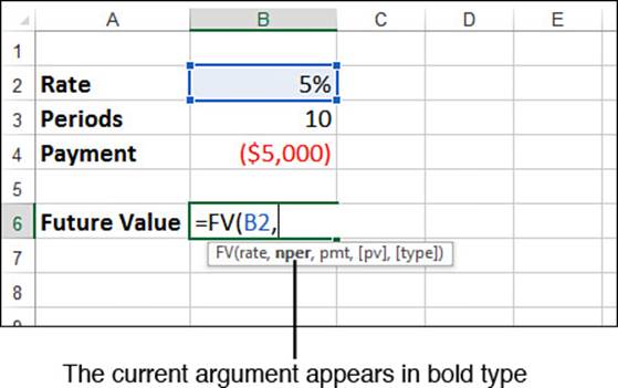
Figure 6.3 After you type the function name and the left parenthesis, Excel displays the function syntax, with the current argument shown in bold type.
Using the Insert Function Feature
Although you’ll usually type your functions by hand, sometimes you might prefer to get a helping hand from Excel, such as in these circumstances:
![]() You’re not sure which function to use.
You’re not sure which function to use.
![]() You want to see the syntax of a function before you use it.
You want to see the syntax of a function before you use it.
![]() You want to examine similar functions in a particular category before you choose the function that best suits your needs.
You want to examine similar functions in a particular category before you choose the function that best suits your needs.
![]() You want to see the effect that different argument values have on the function result.
You want to see the effect that different argument values have on the function result.
For these situations, Excel offers two tools: the Insert Function feature and the Function Wizard.
You use the Insert Function feature to select the function you want from a dialog box. Here’s how it works:
1. Select the cell in which you want to use the function.
2. Enter the formula up to the point where you want to insert the function.
3. Choose one of the following:
• If the function you want is one you inserted recently, it might appear on the list of recent functions in the Name box. Drop down the Name box list (see Figure 6.4); if you see the name of the function you want, click it and skip to step 7.
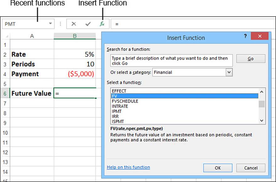
Figure 6.4 Select Formulas, Insert Function or click the Insert Function button to display the Insert Function dialog box.
• To pick any function, select Formulas, Insert Function. (You can also click the Insert Function button in the formula bar—see Figure 6.4—or press Shift+F3.) In this case, the Insert Function dialog box appears, as shown in Figure 6.4.
4. (Optional) In the Or Select a Category list in the Insert Function dialog box, click the type of function you need. If you’re not sure, click All.
5. In the Select a Function list, click the function you want to use. (Note that after you click inside the Select a Function list, pressing a letter moves the selection down to the first function that begins with that letter.)
6. Click OK. Excel displays the Function Arguments dialog box.
Tip
To skip the first six steps and go directly to the Function Arguments dialog box, enter the name of the function and the left parenthesis and then either click the Insert Function button or press Ctrl+A. Alternatively, press the equal sign (=) key and then select the function from the list of recent functions in the Name box. To skip the Function Arguments dialog box altogether, enter the name of the function in the cell and then press Ctrl+Shift+A.
7. For each required argument and each optional argument you want to use, enter a value, an expression, or a cell reference in the appropriate text box. Here are some notes to bear in mind when you’re working in this dialog box (see Figure 6.5):
• The names of the required arguments are shown in bold type.
• When you move the cursor to an argument text box, Excel displays a description of the argument.
• After you fill in an argument text box, Excel shows the current value of the argument to the right of the box.
• After you fill in the text boxes for all the required arguments, Excel displays the current value of the function.
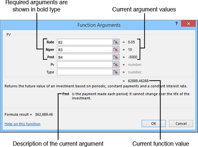
Figure 6.5 Use the Function Arguments dialog box to enter values for a function’s arguments.
8. When you’re finished, click OK. Excel pastes the function and its arguments into the cell.
Loading the Analysis ToolPak
Excel’s Analysis ToolPak is a large collection of powerful statistical tools. Some of these tools use advanced statistical techniques and were designed with only a limited number of technical users in mind. However, many of them have general applications and can be amazingly useful. I go through these tools in several chapters later in the book.
In early versions of Excel (that is, prior to Excel 2007), the Analysis ToolPak included dozens of powerful functions. In Excel 2007 and later, however, all those functions are now part of the Excel function library, so you can use them without loading the Analysis ToolPak.
If you need to use the Analysis ToolPak features, you must load the add-in that makes them available to Excel. The following procedure takes you through the steps:
1. Select File, Options to open the Excel Options dialog box.
2. Click Add-Ins.
3. In the Manage list, click Excel Add-ins and then click Go. Excel displays the Add-Ins dialog box.
4. Select the Analysis ToolPak check box, as shown in Figure 6.6.
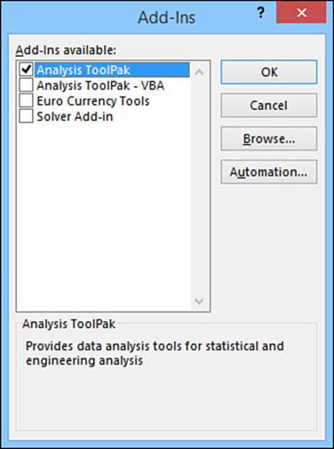
Figure 6.6 Select the Analysis ToolPak check box to load these add-ins into Excel.
5. Click OK.
From Here
![]() For details on Excel’s text-related functions, see Chapter 7, “Working with Text Functions.”
For details on Excel’s text-related functions, see Chapter 7, “Working with Text Functions.”
![]() To learn about the logical and information functions, see Chapter 8, “Working with Logical and Information Functions.”
To learn about the logical and information functions, see Chapter 8, “Working with Logical and Information Functions.”
![]() To get the specifics on Excel’s powerful lookup functions, see Chapter 9, “Working with Lookup Functions.”
To get the specifics on Excel’s powerful lookup functions, see Chapter 9, “Working with Lookup Functions.”
![]() If you want to work with functions related to dates and times, see Chapter 10, “Working with Date and Time Functions.”
If you want to work with functions related to dates and times, see Chapter 10, “Working with Date and Time Functions.”
![]() Excel has a huge library of mathematical functions; see Chapter 11, “Working with Math Functions.”
Excel has a huge library of mathematical functions; see Chapter 11, “Working with Math Functions.”
![]() Excel’s many statistical functions are a powerful tool for data analysis; see Chapter 12, “Working with Statistical Functions.”
Excel’s many statistical functions are a powerful tool for data analysis; see Chapter 12, “Working with Statistical Functions.”
![]() To get the details on functions related to tables, see “Excel’s Table Functions,” p. 313. (Chapter 13)
To get the details on functions related to tables, see “Excel’s Table Functions,” p. 313. (Chapter 13)
![]() For information on using powerful regression functions such as TREND(), LINEST(), and GROWTH(), see Chapter 16, “Using Regression to Track Trends and Make Forecasts.”
For information on using powerful regression functions such as TREND(), LINEST(), and GROWTH(), see Chapter 16, “Using Regression to Track Trends and Make Forecasts.”
![]() Excel has many financial functions related to loans; see Chapter 18, “Building Loan Formulas.”
Excel has many financial functions related to loans; see Chapter 18, “Building Loan Formulas.”
![]() For information on functions related to investments, see Chapter 19, “Building Investment Formulas.”
For information on functions related to investments, see Chapter 19, “Building Investment Formulas.”
![]() To get details on Excel’s discounting functions, see Chapter 20, “Building Discount Formulas.”
To get details on Excel’s discounting functions, see Chapter 20, “Building Discount Formulas.”
All materials on the site are licensed Creative Commons Attribution-Sharealike 3.0 Unported CC BY-SA 3.0 & GNU Free Documentation License (GFDL)
If you are the copyright holder of any material contained on our site and intend to remove it, please contact our site administrator for approval.
© 2016-2026 All site design rights belong to S.Y.A.