Excel® 2016 Formulas and Functions (2016)

Part II: Harnessing the Power of Functions

7. Working with Text Functions

In This Chapter

Excel’s Text Functions

Working with Characters and Codes

Converting Text

Formatting Text

Manipulating Text

Searching for Substrings

Substituting One Substring for Another

In Excel, text is any collection of alphanumeric characters that isn’t a numeric value, a date or time value, or a formula. Words, names, and labels are all obviously text values, but so are cell values preceded by an apostrophe (') or formatted as Text. Text values are also called strings, and I use both terms interchangeably in this chapter.

In Chapter 3, “Building Basic Formulas,” you learned about building text formulas in Excel—not that there was much to learn. Text formulas consist only of the concatenation operator (&) used to combine two or more strings into a larger string.

Excel’s text functions enable you to take text formulas to a more useful level by giving you numerous ways to manipulate strings. With these functions, you can convert numbers to strings, change lowercase letters to uppercase (and vice versa), compare two strings, and more.

Excel’s Text Functions

Table 7.1 summarizes Excel’s text functions, and the rest of this chapter gives you details about and examples of how to use most of them.

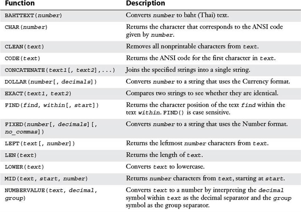
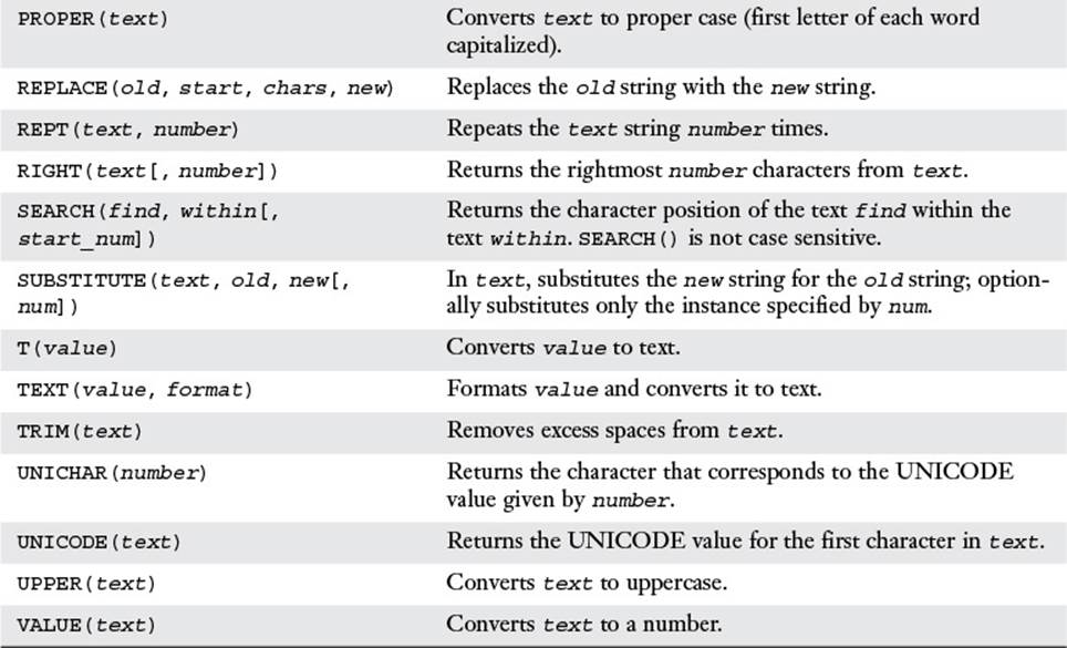
Table 7.1 Excel’s Text Functions

Working with Characters and Codes

Every character you can display on your screen has its own underlying numeric code. For example, the code for the uppercase letter A is 65, whereas the code for the ampersand (&) is 38. These codes apply not only to the alphanumeric characters accessible via your keyboard but also to extra characters. The collection of these characters is called the ANSI character set, and the numbers assigned to each character are called the ANSI codes.

For example, the ANSI code for the copyright character (©) is 169. To display this character, press Alt+0169, where you use your keyboard’s numeric keypad to enter the digits.

Note

When entering digits, remember to always include the leading zero for codes higher than 127.

The ANSI codes run from 1 to 255, although the first 31 codes are nonprinting codes that define characters such as carriage returns and line feeds.

The CHAR() Function

Excel enables you to determine the character represented by an ANSI code using the CHAR() function:

CHAR(number)

For example, the following formula displays the copyright symbol (ANSI code 169):

=CHAR(169)

Note

If you are working with UNICODE values instead of ANSI values, use the UNICHAR() function instead of the CHAR() function.

Generating the ANSI Character Set

Figure 7.1 shows a worksheet that displays the entire ANSI character set, excluding the first 31 nonprinting characters (and note that ANSI code 32 represents the space character). In each case, the character is displayed by applying the CHAR() function to the value in the cell to the left.

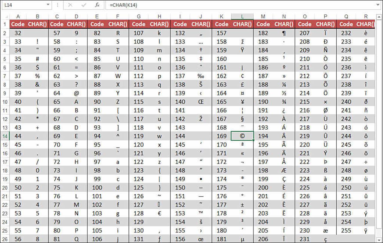
Figure 7.1 This worksheet uses the CHAR() function to display each printing member of the ANSI character set.

Note

The actual character displayed by an ANSI code depends on the font applied to the cell. The characters shown in Figure 7.1 are the ones you see with normal text fonts, such as Arial. However, if you apply a font such as Symbol or Wingdings to the worksheet, you see a different set of characters.

Note

You can download this chapter’s sample workbooks at www.mcfedries.com/books/book.php?title=excel-2016-formulas-and-functions.

To build the character set shown in Figure 7.1, I entered the ANSI code and CHAR() function at the top of each column, and then I filled down to generate the rest of the column. A less tedious method (albeit one with a less useful display) is to take advantage of the ROW() function, which returns the row number of the current cell. Assuming that you want to start your table in row 2, you can generate any ANSI character by using the following formula:

=CHAR(ROW() + 30)

Figure 7.2 shows the results. (The values in column A are generated using the formula =ROW() + 30.)

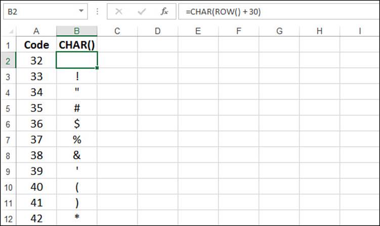
Figure 7.2 This worksheet uses =CHAR(ROW() + 30) to generate the ANSI character set automatically.

Generating a Series of Letters

Excel’s fill handle and Home, Fill, Series command are great for generating a series of numbers or dates, but they don’t do the job when you need a series of letters (such as a, b, c, and so on). However, you can use the CHAR() function in an array formula to generate such a series.

To generate a column of the letters beginning with a (which corresponds to ANSI code 97), enter the following formula where you want the series to begin:

=CHAR(ROW(A97))

To generate a row of the letters beginning with a, enter the following formula where you want the series to begin:

=CHAR(COLUMN(CS1))

Now extend the series by dragging the fill handle down (for a column) or right (for a row).

For uppercase letters (where A corresponds to ANSI 65), begin with the following formulas and use the fill handle to extend the series:

=CHAR(ROW(A65))
=CHAR(COLUMN(BM1))

Figure 7.3 shows these formulas in action.

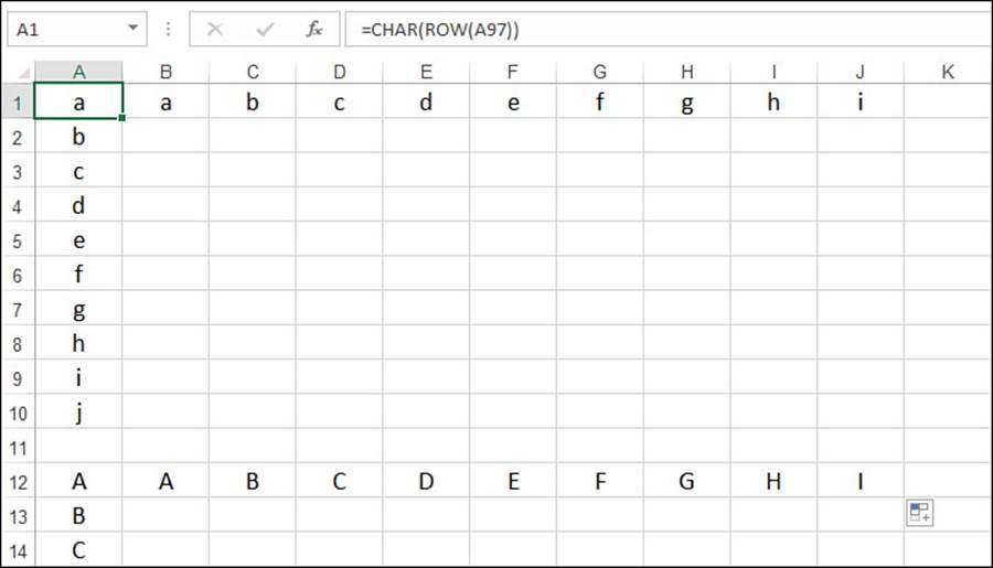
Figure 7.3 Combining the CHAR() and ROW() functions to produce a series of letters.

The CODE() Function

The CODE() function is the opposite of CHAR(). That is, given a text character, CODE() returns its ANSI code value:

CODE(text)

For example, the following formulas both return 83, the ANSI code of the uppercase letter S:

=CODE("S")
=CODE("Spacely Sprockets")

Note

If you need to determine a character’s UNICODE value instead of its ANSI value, use the UNICODE() function instead of the CODE() function.

Generating a Series of Letters Starting from Any Letter

Earlier in this section, you learned how to combine CHAR() and ROW() in an array formula to generate a series of letters beginning with the letter a or A. What if you prefer a different starting letter? You can do that by changing the initial value that’s plugged in to the CHAR() function before the offsets are calculated. I used 97 in the previous example to begin the series with the letter a, but you could use 98 to start with b, 99 to start with c, and so on.

Instead of looking up the ANSI code of the character you prefer, however, use the CODE() function to have Excel do it for you:

=CHAR(CODE("letter") + ROW(range) - ROW(first_cell))

Here, replace letter with the letter you want to start the series with. For example, the following formula begins the series with uppercase N:

=CHAR(CODE("N") + ROW(A1:A13) - ROW(A1))

Tip

When working with the formulas in this section, remember to enter them as array formulas in the specified range.

Converting Text

Excel’s forte is number crunching, and it often seems to give short shrift to strings, particularly when it comes to displaying strings in a worksheet. For example, appending a numeric value to a string results in the number being displayed without any formatting, even if the original cell had a numeric format applied to it. Similarly, strings imported from a database or text file can have the wrong case or no formatting. However, as you’ll see in the next few sections, Excel offers a number of worksheet functions that enable you to convert strings to a more suitable text format or to convert between text and numeric values.

The LOWER() Function

The LOWER() function converts a specified string to all-lowercase letters:

LOWER(text)

For example, the following formula converts the text in cell B10 to lowercase:

=LOWER(B10)

The LOWER() function is often used to convert imported data, particularly data imported from a mainframe computer, which often arrives in all-uppercase characters.

The UPPER() Function

The UPPER() function converts a specified string to all-uppercase letters:

UPPER(text)

For example, the following formula converts the text in cells A5 and B5 to uppercase and concatenates the results with a space between them:

=UPPER(A5) & " " & UPPER(B5)

The PROPER() Function

The PROPER() function converts a specified string to proper case, which means the first letter of each word appears in uppercase and the rest of the letters appear in lowercase:

PROPER(text)

For example, the following formula, entered as an array, converts the text in the range A1:A10 to proper case:

=PROPER(A1:A10)

The NUMBERVALUE() Function

The NUMBERVALUE() function, which was introduced in Excel 2013, converts a text value to a number by specifying the symbol used for the decimal and groups:

NUMBERVALUE(text[, decimal_separator][, group_separator])

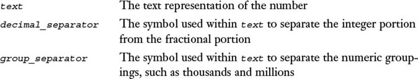
This function is useful if you’re faced with a worksheet that contains numbers that use nonstandard symbols for the decimal and group separators. For example, suppose cell C6 contains 12,34, where the comma (,) is being used as a decimal separator (which is common in many European locales). To convert this value to a number that uses a period (assuming that’s your local decimal separator symbol), you’d use the following formula:

=NUMBERVALUE(C6, ",")

As another example, suppose cell E5 contains the value 2~345'67, where tilde (~) is the group (thousands, in this case) separator and apostrophe (') is the decimal separator. Then the following formula converts this value to a number:

=NUMBERVALUE(E5, "'", "~")

Formatting Text

You learned in Chapter 3 that you can enhance the results of your formulas by using built-in or custom numeric formats to control things such as commas, decimal places, currency symbols, and more. That’s fine for cell results, but what if you want to incorporate a result within a string? For example, consider the following text formula:

="The expense total for this quarter in 2015 is " & F11

No matter how you’ve formatted the result in F11, the number appears in the string using Excel’s General number format. For example, if cell F11 contains $74,400, the previous formula will appear in the cell as follows:

The expense total for this quarter in 2015 is 74400

You need some way to format the number within the string. The next three sections show you some Excel functions that let you do just that.

The DOLLAR() Function

The DOLLAR() function converts a numeric value into a string value that uses the Currency format:

DOLLAR(number [,decimals])

To fix the string example from the previous section, you need to apply the DOLLAR() function to cell F11:

="The expense total for this quarter in 2015 is " & DOLLAR(F11, 0)

In this case, the number is formatted with no decimal places. Figure 7.4 shows a variation of this formula in action in cell B16. (The original formula is shown in cell B15.)

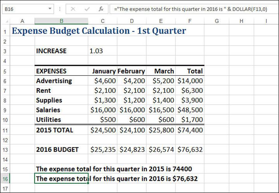
Figure 7.4 Use the DOLLAR() function to display a number as a string with the Currency format.

The FIXED() Function

For some kinds of numbers, you can control the number of decimals and whether commas are inserted as the thousands separator by using the FIXED() function:

FIXED(number [,decimals] [,no_commas])

For example, the following formula uses the SUM() function to take a sum over a range and applies the FIXED() function to the result so that it is displayed as a string with commas and no decimal places:

="Total show attendance: " & FIXED(SUM(A1:A8), 0, FALSE) & " people."

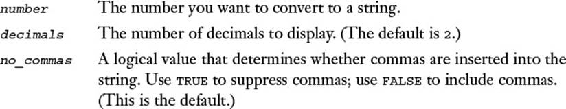
The TEXT() Function

DOLLAR() and FIXED() are useful functions in specific circumstances. However, if you want total control over the way a number is formatted within a string, or if you want to include dates and times within strings, the powerful TEXT() function is what you need:

TEXT(number, format)

The power of the TEXT() function lies in its format argument, which is a custom format that specifies exactly how you want the number to appear. You learned about building custom numeric, date, and time formats back in Chapter 3.

To learn about custom numeric formatting, see “Customizing Numeric Formats,” p. 78.

To learn about custom date and time formatting, see “Customizing Date and Time Formats,” p. 84.

For example, the following formula uses the AVERAGE() function to take an average over the range A1:A31, and then it uses the TEXT() function to apply the custom format #,##0.00°F to the result:

="The average temperature was " & TEXT(AVERAGE(A1:A31), "#,##0.00°F")

Note

To insert the degree symbol (°), type Alt+0176 using your keyboard’s numeric keypad.

Displaying When a Workbook Was Last Updated

Many people like to annotate their workbooks by setting Excel in manual calculation mode and entering a NOW() function into a cell (which returns the current date and time). The NOW() function doesn’t update unless you save or recalculate the sheet, so you always know when the sheet was last updated.

Instead of just entering NOW() by itself, you might find it better to preface the date with an explanatory string, such as This workbook last updated:. To do this, you can enter the following formula:

="This workbook last updated: " & NOW()

Unfortunately, your output will look something like this:

This workbook last updated: 42238.51001

The number 42238.51001 is Excel’s internal representation of a date and time. (The number to the left of the decimal is the date, and the number to the right of the decimal is the time.) To get a properly formatted date and time, use the TEXT() function. For example, to format the results of the NOW() function in the MM/DD/YY HH:MM format, use the following formula:

="This workbook last updated: " & TEXT(NOW(), "mm/dd/yy hh:mm")

Manipulating Text

The rest of this chapter takes you into the real heart of Excel’s text-manipulation tricks. All the functions you’ll learn about over the next few pages will be useful, but you’ll see that by combining two or more of these functions into a single formula, you can bring out the amazing versatility of Excel’s text-manipulation prowess.

Removing Unwanted Characters from a String

Characters imported from databases and text files often come with all kinds of string baggage in the form of extra characters that you don’t need. These could be extra spaces in the string, or they could be line feeds, carriage returns, and other nonprintable characters embedded in the string. To fix these problems, Excel offers a couple functions: TRIM() and CLEAN().

The TRIM() Function

You use the TRIM() function to remove excess spaces within a string:

TRIM(text)

Here, excess means all spaces before and after the string, as well as two or more consecutive spaces within the string. In the latter case, TRIM() removes all but one of the consecutive spaces.

Figure 7.5 shows the TRIM() function at work. Each string in the range A2:A7 contains a number of excess spaces before, within, or after the name. The TRIM() functions appear in column C. To help confirm the TRIM() function’s operation, I use the LEN() text function in columns B and D. LEN() returns the number of characters in a specified string, using the following syntax:

LEN(text)

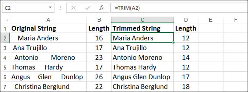
Figure 7.5 Use the TRIM() function to remove extra spaces from a string.

The CLEAN() Function

You use the CLEAN() function to remove nonprintable characters from a string:

CLEAN(text)

Recall that the nonprintable characters are the codes 1 through 31 of the ANSI character set. The CLEAN() function is most often used to remove line feeds (ANSI 10) or carriage returns (ANSI 13) from multiline data. Figure 7.6 shows an example.

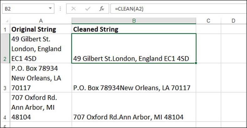
Figure 7.6 Use the CLEAN() function to remove nonprintable characters such as line feeds from a string.

The REPT() Function: Repeating a Character or String

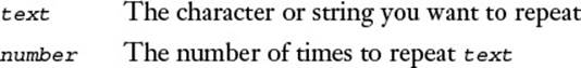
The REPT() function repeats a character or string a specified number of times:

REPT(text, number)

Padding a Cell

The REPT() function is sometimes used to pad a cell with characters. For example, you can use it to add leading or trailing dots in a cell. Here’s a formula that creates trailing dots after a string:

="Advertising" & REPT(".", 20 - LEN("Advertising"))

This formula writes the string Advertising and then uses REPT() to repeat the dot character according to the following expression: 20 - LEN("Advertising"). This expression ensures that characters are written to the cell. Because Advertising is 11 characters, the expression result is 9, which means that nine dots are added to the right of the string. If the string were Rent (four characters) instead, 16 dots would be added as padding. Figure 7.7 shows how this technique creates a dot follower effect.

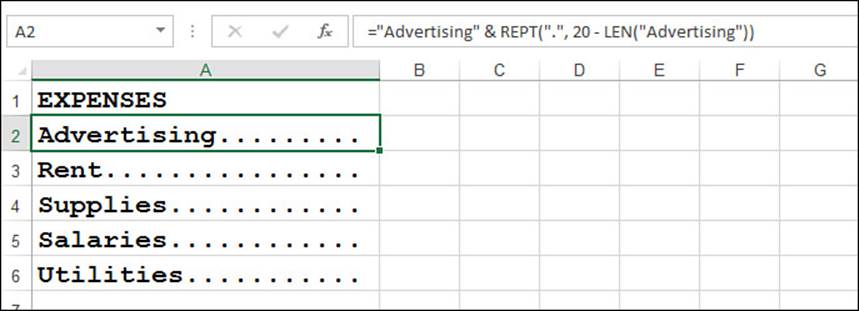
Figure 7.7 Use the REPT() function to pad a cell with characters, such as the dot followers shown here.

Tip

For best results, the cells need to be formatted in a monotype font, such as Courier New. This ensures that all characters are the same width, which gives you consistent results in all the cells.

Building Text Charts

A more common use for the REPT() function is to build text-based charts. In this case, you use a numeric result in a cell as the REPT() function’s number argument, and the repeated character then charts the result.

A simple example is a basic histogram, which shows the frequency of a sample over an interval. Figure 7.8 shows a text histogram in which the intervals are listed in column A and the frequencies are listed in column B. The REPT() function creates the histogram in column C by repeating the vertical bar (|) according to each frequency, as in this sample formula:

=REPT("|", B4)

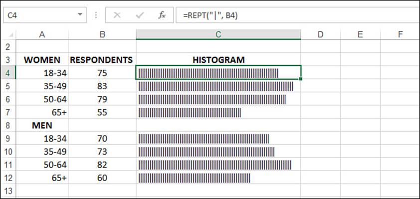
Figure 7.8 Use the REPT() function to create a text-based histogram.

With a simple trick, you can turn the histogram into a text-based bar chart, as shown in Figure 7.9. The trick here is to format the chart cells with the Webdings font. In this font, the letter g is represented by a block character, and repeating that character produces a solid bar.

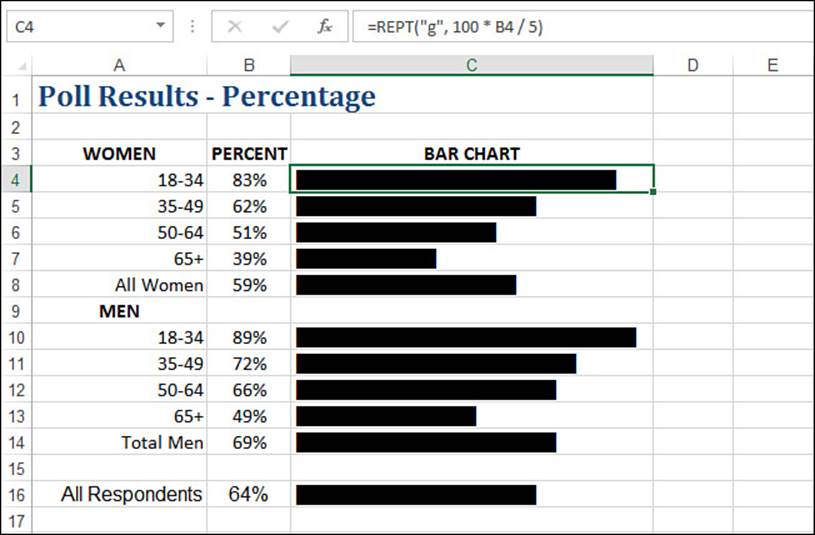
Figure 7.9 Use the REPT() function to create a text-based bar chart.

Tip

To get the repeat value, I multiplied the percentages in column B by 100 to get a whole number. To keep the bars relatively short, I divided the result by 5.

Excel offers a feature called data bars that enables you to easily add histogram-like analysis to your worksheets without formulas. See “Adding Data Bars,” p. 29.

Extracting a Substring

String values often contain smaller strings, or substrings, that you need to work with. In a column of full names, for example, you might want to deal with only the last names so that you can sort the data. Similarly, you might want to extract the first few letters of a company name to include in an account number for that company.

Excel gives you three functions for extracting substrings, as described in the next three sections.

The LEFT() Function

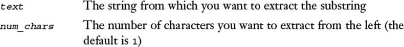
The LEFT() function returns a specified number of characters, starting from the left of a string:

LEFT(text [,num_chars])

For example, the following formula returns the substring Karen:

=LEFT("Karen Elizabeth McHammond", 5)

The RIGHT() Function

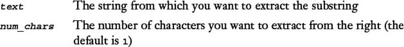
The RIGHT() function returns a specified number of characters, starting from the right of a string:

RIGHT(text [,num_chars])

For example, the following formula returns the substring McHammond:

=RIGHT("Karen Elizabeth McHammond", 9)

The MID() Function

The MID() function returns a specified number of characters starting from any point within a string:

MID(text, start_num, num_chars)

For example, the following formula returns the substring Elizabeth:

=MID("Karen Elizabeth McHammond", 7, 9)

Converting Text to Sentence Case

Microsoft Word’s Change Case command has a sentence case option that converts a string to all-lowercase letters, except for the first letter, which is converted to uppercase (just as the letters would appear in a normal sentence). You saw earlier that Excel has LOWER(), UPPER(), andPROPER() functions, but it has nothing that can produce sentence case directly. However, it’s possible to construct a formula that does this, by using the LOWER() and UPPER() functions combined with the LEFT() and RIGHT() functions.

You begin by extracting the leftmost letter and converting it to uppercase (assuming here that the string is in cell A1):

UPPER(LEFT(A1))

Then you extract everything to the right of the first letter and convert it to lowercase:

LOWER(RIGHT(A1, LEN(A1) - 1))

Finally, you concatenate these two expressions into the complete formula:

=UPPER(LEFT(A1)) & LOWER(RIGHT(A1, LEN(A1) - 1))

Figure 7.10 shows a worksheet that puts this formula through its paces.

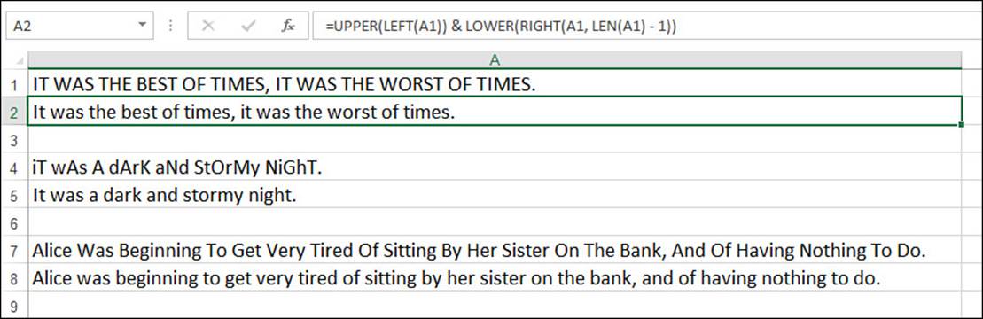
Figure 7.10 The LEFT() and RIGHT() functions combine with the UPPER() and LOWER() functions to produce a formula that converts text to sentence case.

A Date-Conversion Formula

If you import mainframe or server data into your worksheets, or if you import online service data such as stock market quotes, you’ll often end up with date formats that Excel can’t handle. One common example is the YYYYMMDD format (for example, 20160823).

To convert this value into a date that Excel can work with, you can use the LEFT(), MID(), and RIGHT() functions. If the unrecognized date is in cell A1, LEFT(A1, 4) extracts the year, MID(A1,5,2) extracts the month, and RIGHT(A1,2) extracts the day. Plugging these functions into a DATE() function gives Excel a date it can handle:

=DATE(LEFT(A1, 4), MID(A1, 5, 2), RIGHT(A1, 2))

To learn more about the DATE() function, see “DATE(): Returning Any Date,” p. 212.

Case Study: Generating Account Numbers, Part I

Many companies generate supplier or customer account numbers by combining part of an account’s name with a numeric value. Excel’s text functions make it easy to generate such account numbers automatically.

To begin, let’s extract the first three letters of the company name and convert them to uppercase for easier reading (assuming here that the name is in cell A2):

UPPER(LEFT(A2, 3))

Next, generate the numeric portion of the account number by grabbing the row number: ROW(A2). However, it’s best to keep all account numbers a uniform length, so use the TEXT() function to pad the row number with zeros:

TEXT(ROW(A2), "0000")

Here’s the complete formula, and Figure 7.11 shows some examples:

=UPPER(LEFT(A2, 3)) & TEXT(ROW(A2), "0000")

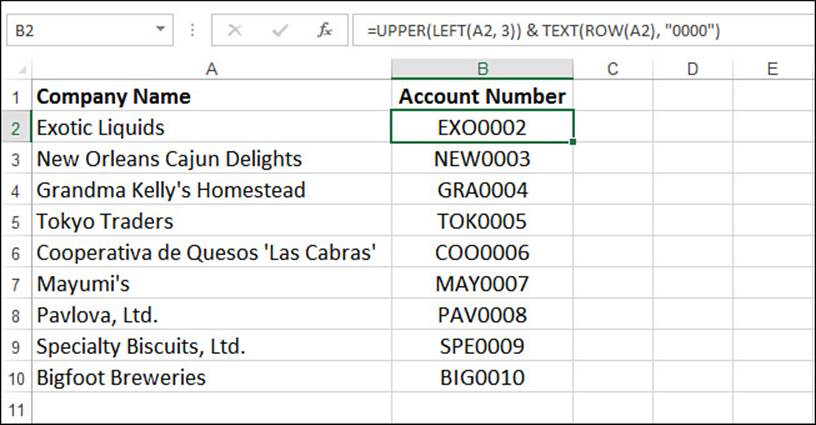
Figure 7.11 This worksheet uses the UPPER(), LEFT(), and TEXT() functions to automatically generate account numbers from company names.

Searching for Substrings

You can take Excel’s text functions up a notch or two by searching for substrings within some given text. For example, in a string that includes a person’s first and last names, you can find out where the space falls between the names and then use that fact to extract either the first name or the last name.

The FIND() and SEARCH() Functions

Searching for substrings is handled by the FIND() and SEARCH() functions:

FIND(find_text, within_text [,start_num])
SEARCH(find_text, within_text [,start_num])

Here are some notes to bear in mind when using these functions:

These functions return the character position of the first instance (after the start_num character position) of find_text in within_text.

Use SEARCH() for non-case-sensitive searches. For example, SEARCH("e", "Expenses") returns 1.

Use FIND() for case-sensitive searches. For example, FIND("e", "Expenses") returns 4.

These functions return the #VALUE! error if find_text is not in within_text.

In the find_text argument of SEARCH(), use a question mark (?) to match any single character.

In the find_text argument of SEARCH(), use an asterisk (*) to match any number of characters.

To include the character ? or * in a SEARCH() operation, precede each instance in the find_text argument with a tilde (~). If you want to search for a tilde character, use two tildes (~~).

Extracting a First Name or Last Name

If you have a range of cells containing people’s first and last names, it can often be advantageous to extract these names from each string. For example, you might want to store the first and last names in separate ranges for later importing into a database table. Or perhaps you need to construct a new range using a Last Name, First Name structure for sorting the names.

The solution is to use the FIND() function to find the space that separates the first and last names and then use either the LEFT() function to extract the first name or the RIGHT() function to extract the last name.

Remember that Excel 2016 offers the Flash Fill feature, which is usually easier for tasks such as extracting names. See “Flash-Filling a Range,” p. 18.

For the first name, you use the following formula (assuming that the full name is in cell A2):

=LEFT(A2, FIND(" ", A2) - 1)

Notice that the formula subtracts 1 from the FIND(" ", A2) result to avoid including the space in the extracted substring. You can use this formula in more general circumstances to extract the first word of any multiword string.

For the last name, you need to build a similar formula using the RIGHT() function:

=RIGHT(A2, LEN(A2) - FIND(" ", A2))

To extract the correct number of letters, the formula takes the length of the original string and subtracts the position of the space. You can use this formula in more general circumstances to extract the second word in any two-word string.

Figure 7.12 shows a worksheet that puts both formulas to work.

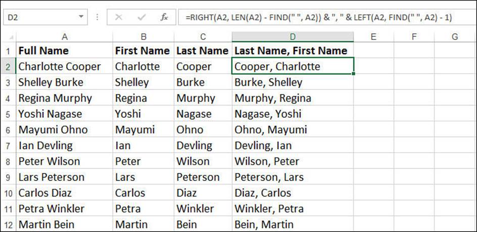
Figure 7.12 Use the LEFT() and FIND() functions to extract the first name; use the RIGHT() and FIND() functions to extract the last name.

Caution

These formulas cause an error in any string that contains only a single word. To allow for this, use the IFERROR() function:

=IFERROR(LEFT(A2, FIND(" ", A2) - 1), A2)

This way, if the cell contains a space, all is well, and the formula runs normally. If the cell does not contain a space, the FIND() function returns an error. Therefore, instead of returning the formula result, the IFERROR() function returns just the cell text (A2).

Extracting First Name, Last Name, and Middle Initial

If the full name you have to work with includes the person’s middle initial, the formula for extracting the first name remains the same. However, you need to adjust the formula for finding the last name. There are a couple ways to go about this, but the method I’m showing you utilizes a useful FIND() and SEARCH() trick. Specifically, if you want to find the second instance of a substring, start the search one character position after the first instance of the substring. Here’s an example of a string:

Karen E. McHammond

Assuming that this string is in A2, the formula =FIND(" ", A2) returns 6, the position of the first space. If you want to find the position of the second space, instead set the FIND() function’s start_num argument to 7—or, more generally, to the location of the first space, plus 1:

=FIND(" ", A2, FIND(" ",A2) + 1)

You can then apply this result within the RIGHT() function to extract the last name:

=RIGHT(A2, LEN(A2) - FIND(" ", A2, FIND(" ", A2) +1))

To extract the middle initial, search for the period (.) and use MID() to extract the letter before it:

=MID(A2, FIND(".", A2) - 1, 1)

Figure 7.13 shows a worksheet that demonstrates these techniques.

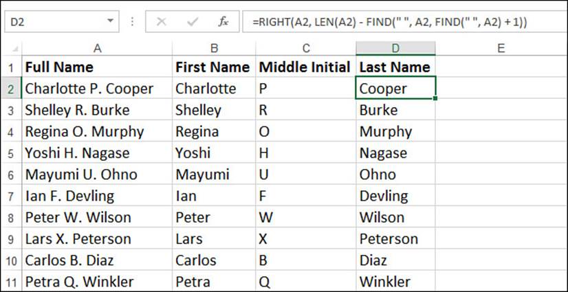
Figure 7.13 Apply FIND() after the first instance of a substring to find the second instance of the substring.

Determining the Column Letter

Excel’s COLUMN() function returns the column number of a specified cell. For example, for a cell in column A, COLUMN() returns 1. This is handy, as you saw earlier in this chapter (“Generating a Series of Letters”), but in some cases you might prefer to know the actual column letter.

This is a tricky proposition because the letters run from A to Z, then AA to AZ, and so on. However, Excel’s CELL() function can return (among other things) the address of a specified cell in absolute format—for example, $A$2 or $AB$10. To get the column letter, you need to extract the substring between the two dollar signs. It’s clear to begin with that the substring will always start at the second character position, so we can begin with the following formula:

=MID(CELL("Address", A2), 2, num_chars)

To learn more about the CELL() function, see “The CELL() Function,” p. 182.

The num_chars value will be either 1, 2, or 3, depending on the column. Notice, however, that the position of the second dollar sign will either be 3, 4, or 5, depending on the column. In other words, the length of the substring will always be two less than the position of the second dollar sign. So, the following expression will give the num_chars value:

FIND("$", CELL("address",A2), 3) - 2

Here, then, is the full formula:

=MID(CELL("Address", A2), 2, FIND("$", CELL("address", A2), 3) - 2)

Getting the column letter of the current cell requires a slightly shorter formula:

=MID(CELL("Address"), 2, FIND("$", CELL("address"), 3) - 2)

Substituting One Substring for Another

The Office programs (and indeed most Windows programs) come with a Replace command that enables you to search for some text and then replace it with some other string. Excel’s collection of worksheet functions also comes with such a feature, in the guise of the REPLACE() andSUBSTITUTE() functions.

The REPLACE() Function

Here’s the syntax of the REPLACE() function:

REPLACE(old_text, start_num, num_chars, new_text)

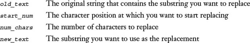
The tricky parts of this function are the start_num and num_chars arguments. How do you know where to start and how much to replace? This isn’t hard if you know the original string in which the replacement is going to take place and if you know the replacement string. For example, consider the following string:

Expense Budget for 2015

To replace 2015 with 2016, and assuming that the string is in cell A1, the following formula does the job:

=REPLACE(A1, 20, 4, "2016")

However, it’s a pain to have to calculate by hand the start_num and num_chars arguments. And in more general situations, you might not even know these values. Therefore, you need to calculate them:

To determine the start_num value, use the FIND() or SEARCH() function to locate the substring you want to replace.

To determine the num_chars value, use the LEN() function to get the length of the replacement text.

The revised formula then looks something like this (assuming that the original string is in A1 and the replacement string is in A2):

=REPLACE(A1, FIND("2015", A1), LEN("2015"), A2)

The SUBSTITUTE() Function

The extra steps required make the REPLACE() function unwieldy, so most people use the more straightforward SUBSTITUTE() function:

SUBSTITUTE(text, old_text, new_text [,instance_num])

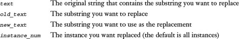
The following simpler formula does the same thing as the example in the previous section:

=SUBSTITUTE(A1, "2015", "2016")

Removing a Character from a String

Earlier, you learned about the CLEAN() function, which removes nonprintable characters from a string, as well as the TRIM() function, which removes excess spaces from a string. A common text scenario involves removing all instances of a particular character from a string. For example, you might want to remove spaces from a string or an apostrophe from a name.

Here’s a generic formula that does this:

=SUBSTITUTE(text, character, "")

Here, replace text with the original string and character with the character you want to remove. For example, the following formula removes all the spaces from the string in cell A1:

=SUBSTITUTE(A1, " ", "")

Note

One surprising use of the SUBSTITUTE() function is to count the number of characters that appear in a string. The trick here is that if you remove a particular character from a string, the difference in length between the original string and the resulting string is the same as the number of times the character appeared in the original string. For example, the string expenses has eight characters. If you remove all the e’s, the resulting string is xpnss, which has five characters. The difference is 3, which is how many e’s there were in the original string.

To calculate this in a formula, use the LEN() function and subtract the length of a string with the character removed from the length of the original string. Here’s the formula that counts the number of e’s for a string in cell A1:

=LEN(A1) - LEN(SUBSTITUTE(A1, "e", ""))

Removing Two Different Characters from a String

It’s possible to nest one SUBSTITUTE() function inside another to remove two different characters from a string. For example, first consider the following expression, which uses SUBSTITUTE() to remove periods from a string:

SUBSTITUTE(A1, ".", "")

Because this expression returns a string, you can use that result as the text argument in another SUBSTITUTE() function. Here, then, is a formula that removes both periods and spaces from a string in cell A1:

=SUBSTITUTE(SUBSTITUTE(A1, ".", ""), " ", "")

Case Study: Generating Account Numbers, Part II

The formula I showed you earlier for automatically generating account numbers from an account name produces valid numbers only if the first three letters of the name are letters. If you have names that contain characters other than letters, you need to remove those characters before generating the account number. For example, if you have an account name such as J. D. BigBelly, you need to remove periods and spaces before generating the account name. You can do this by adding the expression from the previous section to the formula for generating an account name from earlier in this chapter. Specifically, you replace the cell address in LEFT() with the nested SUBSTITUTE() functions, as shown in Figure 7.14. Notice that the formula still works on account names that begin with three letters.

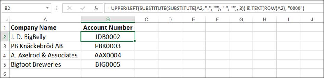
Figure 7.14 This worksheet uses nested SUBSTITUTE() functions to remove periods and spaces from account names before generating the account numbers.

Removing Line Feeds

Earlier in this chapter, you learned about the CLEAN() function, which removes nonprintable characters from a string. In the example, I used CLEAN() to remove the line feeds from a multiline cell entry. However, you might have noticed a small problem with the result: There was no space between the end of one line and the beginning of the next line (refer to Figure 7.6).

If all you’re worried about is line feeds, use the following SUBSTITUTE() formula instead of the CLEAN() function:

=SUBSTITUTE(A2, CHAR(10), " ")

This formula replaces the line feed character (ANSI code 10) with a space, resulting in a proper string, as shown in Figure 7.15.

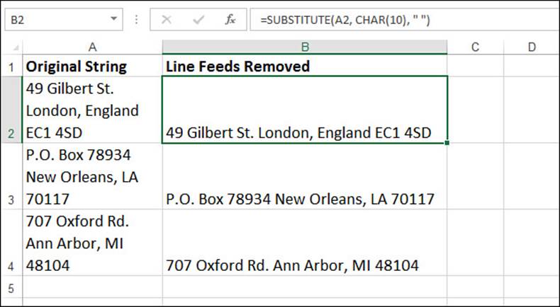
Figure 7.15 This worksheet uses SUBSTITUTE() to replace each line feed character with a space.

From Here

For details on custom formatting, see “Formatting Numbers, Dates, and Times,” p. 74.

For a general discussion of function syntax, see “The Structure of a Function,” p. 130.

To learn more about the CELL() function, see “The CELL() Function,” p. 182.

To learn more about the DATE() function, see “DATE(): Returning Any Date,” p. 212.