Excel® 2016 Formulas and Functions (2016)
Part II: Harnessing the Power of Functions
9. Working with Lookup Functions
In This Chapter
Excel’s Lookup Functions
Understanding Lookup Tables
The CHOOSE() Function
Looking Up Values in Tables
Getting the meaning of a word in the dictionary is always a two-step process: First you look up the word itself, and then you read its definition. Same with an encyclopedia: First look up the concept, and then you read the article.
This idea of looking something up to retrieve some related information is at the heart of many spreadsheet operations. For example, you saw in Chapter 4, “Creating Advanced Formulas,” that you can add option buttons and list boxes to a worksheet. Unfortunately, these controls return only the number of the item the user has chosen. To find out the actual value of the item, you need to use the returned number to look up the value in a table.
![]() For the specifics of adding option buttons and list boxes to a worksheet, see “Understanding the Worksheet Controls,” p. 105.
For the specifics of adding option buttons and list boxes to a worksheet, see “Understanding the Worksheet Controls,” p. 105.
Excel’s Lookup Functions
In many worksheet formulas, the value of one argument often depends on the value of another. Here are some examples:
![]() In a formula that calculates an invoice total, the customer’s discount might depend on the number of units purchased.
In a formula that calculates an invoice total, the customer’s discount might depend on the number of units purchased.
![]() In a formula that charges interest on overdue accounts, the interest percentage might depend on the number of days each invoice is overdue.
In a formula that charges interest on overdue accounts, the interest percentage might depend on the number of days each invoice is overdue.
![]() In a formula that calculates employee bonuses as a percentage of salary, the percentage might depend on how much the employee improved on the given budget.
In a formula that calculates employee bonuses as a percentage of salary, the percentage might depend on how much the employee improved on the given budget.
The usual way to handle these kinds of problems is to look up the appropriate value. This chapter introduces you to a number of functions that enable you to perform lookup operations in your worksheet models. Table 9.1 lists Excel’s lookup functions.
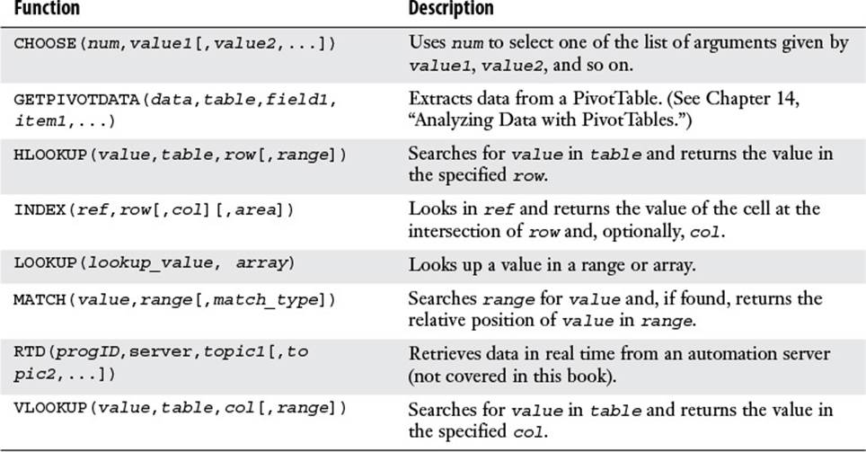
Table 9.1 Excel’s Lookup Functions
Understanding Lookup Tables
The table—more properly referred to as a lookup table—is the key to performing lookup operations in Excel. The most straightforward lookup table structure is one that consists of two columns (or two rows):
![]() Lookup column—This column contains the values that you look up. For example, if you were constructing a lookup table for a dictionary, this column would contain the words.
Lookup column—This column contains the values that you look up. For example, if you were constructing a lookup table for a dictionary, this column would contain the words.
![]() Data column—This column contains the data associated with each lookup value. In the dictionary example, this column would contain the definitions.
Data column—This column contains the data associated with each lookup value. In the dictionary example, this column would contain the definitions.
In most lookup operations, you supply a value that the function locates in the designated lookup column. It then retrieves the corresponding value in the data column.
As you’ll see in this chapter, there are many variations on the lookup table theme. The lookup table can be one of these:
![]() A single column (or a single row)—In this case, the lookup operation consists of finding the nth value in the column.
A single column (or a single row)—In this case, the lookup operation consists of finding the nth value in the column.
![]() A range with multiple data columns—For instance, in the dictionary example, you might have a second column for each word’s part of speech (noun, verb, and so on), and perhaps a third column for its pronunciation. In this case, the lookup operation must also specify which of the data columns contains the value required.
A range with multiple data columns—For instance, in the dictionary example, you might have a second column for each word’s part of speech (noun, verb, and so on), and perhaps a third column for its pronunciation. In this case, the lookup operation must also specify which of the data columns contains the value required.
![]() An array—In this case, the table doesn’t exist on a worksheet but is either an array of literal values or the result of a function that returns an array. The lookup operation finds a particular position within the array and returns the data value at that position.
An array—In this case, the table doesn’t exist on a worksheet but is either an array of literal values or the result of a function that returns an array. The lookup operation finds a particular position within the array and returns the data value at that position.
The CHOOSE() Function
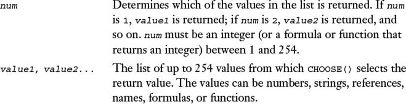
The simplest of the lookup functions is CHOOSE(), which enables you to select a value from a list. Specifically, given an integer n, CHOOSE() returns the nth item from the list. Here’s the function’s syntax:
CHOOSE(num, value1[, value2,...])
For example, consider the following formula:
=CHOOSE(2,"Surface Mail", "Air Mail", "Courier")
The num argument is 2, so CHOOSE() returns the second value in the list, which is the string value Air Mail.
Note
If you use range references as the list of values, CHOOSE() returns the entire range as the result. For example, consider the following:
CHOOSE(1, A1:D1, A2:D2, A3:D3)
This function returns the range A1:D1. This enables you to perform conditional operations on a set of ranges, where the condition is the lookup value used by CHOOSE(). For example, the following formula returns the sum of the range A1:D1:
=SUM(CHOOSE(1, A1:D1, A2:D2, A3:D3))
Determining the Name of the Day of the Week
As you’ll see in Chapter 10, “Working with Date and Time Functions,” Excel’s WEEKDAY() function returns a number that corresponds to the day of the week, where Sunday is 1, Monday is 2, and so on.
![]() To learn about the WEEKDAY() function, see “The WEEKDAY() Function,” p. 214.
To learn about the WEEKDAY() function, see “The WEEKDAY() Function,” p. 214.
What if you want to know the actual day (not the number) of the week? If you need only to display the day of the week, you can format the cell as dddd. If you need to use the day of the week as a string value in a formula, you need a way to convert the WEEKDAY() result into the appropriate string. Fortunately, the CHOOSE() function makes this process easy. For example, suppose that cell B5 contains a date. You can find the day of the week it represents with the following formula:
=CHOOSE(WEEKDAY(B5), "Sun", "Mon", "Tue", "Wed", "Thu", "Fri", "Sat")
I’ve used abbreviated day names to save space, but you’re free to use any form of the day names that suits your purposes.
Note
Here’s a similar formula for returning the name of the month, given the integer month number returned by the MONTH() function:
=CHOOSE(MONTH(date), "Jan", "Feb", "Mar", "Apr", "May",
"Jun", "Jul", "Aug", "Sep", "Oct", "Nov", "Dec")
Determining the Month of the Fiscal Year
For many businesses, the fiscal year does not coincide with the calendar year. For example, the fiscal year might run from April 1 to March 31. In this case, month 1 of the fiscal year is April, month 2 is May, and so on. It’s often handy to be able to determine the fiscal month, given the calendar month.
To see how you’d set this up, first consider the following table, which compares the calendar month and the fiscal month for a fiscal year beginning April 1:
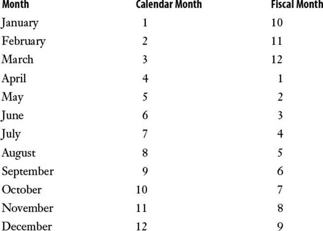
You need to use the calendar month as the lookup value and the fiscal months as the data values. Here’s the result:
=CHOOSE(CalendarMonth, 10, 11, 12, 1, 2, 3, 4, 5, 6, 7, 8, 9)
Figure 9.1 shows an example.
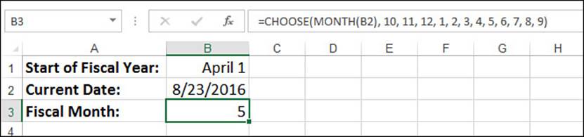
Figure 9.1 This worksheet uses the CHOOSE() function to determine the fiscal month (B3), given the start of the fiscal year (shown in B1) and the current date (B2).
Note
You can download this chapter’s sample workbook at www.mcfedries.com/books/book.php?title=excel-2016-formulas-and-functions.
Calculating Weighted Questionnaire Results
One common use for CHOOSE() is to calculate weighted questionnaire responses. For example, suppose that you just completed creating a survey in which the respondents have to enter a value between 1 and 5 for each question. Some questions and answers are more important than others, so each question is assigned a set of weights. You use these weighted responses for your data. How do you assign the weights? The easiest way is to set up a CHOOSE() function for each question. For instance, suppose that question 1 uses the following weights for answers 1 through 5: 1.5, 2.3, 1.0, 1.8, and 0.5. If so, the following formula can be used to derive the weighted response:
=CHOOSE(Answer1, 1.5, 2.3, 1.0, 1.8, 0.5)
Assume that the answer for question 1 is in a cell named Answer1.
Integrating CHOOSE() and Worksheet Option Buttons
The CHOOSE() function is ideal for lookup situations in which you have a small number of data values and you have a formula or function that generates sequential integer values beginning with 1. A good example of this is the use of the worksheet option buttons I mentioned at the beginning of this chapter. The option buttons in a group return integer values in the linked cell: 1 if the first option is clicked, 2 if the second option is clicked, and so on. Therefore, you can use the value in the linked cell as the lookup value in the CHOOSE() function. Figure 9.2 shows a worksheet that does this.
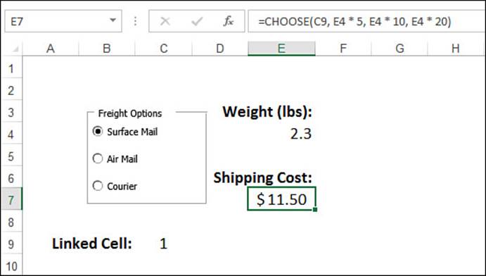
Figure 9.2 This worksheet uses the CHOOSE() function to calculate the shipping cost based on the option clicked in the Freight Options group.
The Freight Options group presents three option buttons: Surface Mail, Air Mail, and Courier. The number of the currently selected option is shown in the linked cell, C9. A weight, in pounds, is entered into cell E4. Given the linked cell and the weight, cell E7 calculates the shipping cost by using CHOOSE() to select a formula that multiplies the weight by a constant:
=CHOOSE(C9, E4 * 5, E4 * 10, E4 * 20)
Looking Up Values in Tables
As you’ve seen, the CHOOSE() function is a handy and useful addition to your formula toolkit, and it’s a function you’ll turn to quite often if you build a lot of worksheet models. However, CHOOSE() does have its drawbacks:
![]() The lookup values must be positive integers.
The lookup values must be positive integers.
![]() The maximum number of data values is 254.
The maximum number of data values is 254.
![]() Only one set of data values is allowed per function.
Only one set of data values is allowed per function.
You’ll trip over these limitations eventually, and you’ll wonder if Excel has more flexible lookup capabilities. Can it use a wider variety of lookup values (negative or real numbers, strings, and so on)? Can it accommodate multiple data sets that each can have any number of values (subject, of course, to the worksheet’s inherent size limitations)? The answer to both questions is “yes”; in fact, Excel has two functions that meet these criteria: VLOOKUP() and HLOOKUP().
The VLOOKUP() Function
The VLOOKUP() function works by looking in the first column of a table for the value you specify. (The V in VLOOKUP() stands for vertical.) It then looks across the appropriate number of columns (which you specify) and returns whatever value it finds there.
Here’s the full syntax for VLOOKUP():
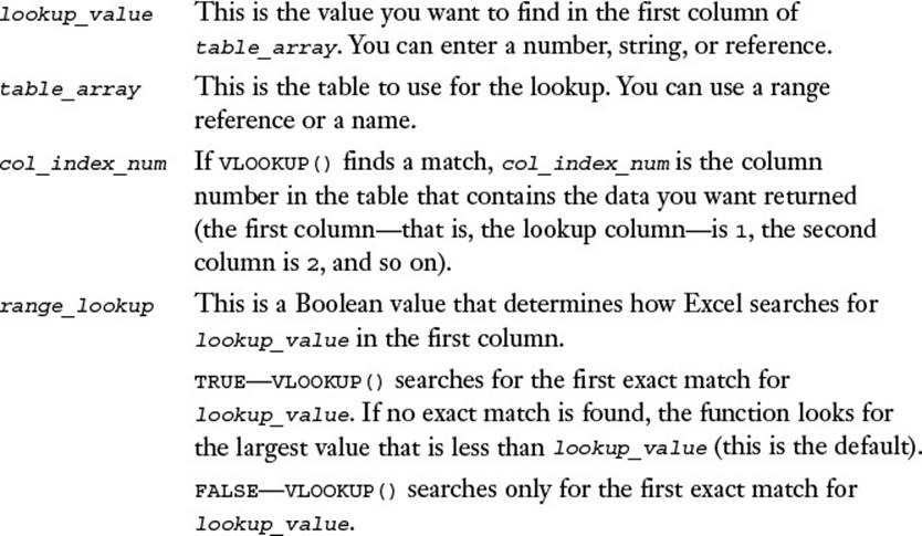
VLOOKUP(lookup_value, table_array, col_index_num[, range_lookup])
Here are some notes to keep in mind when you work with VLOOKUP():
![]() If range_lookup is TRUE or omitted, you must sort the values in the first column in ascending order.
If range_lookup is TRUE or omitted, you must sort the values in the first column in ascending order.
![]() If the first column of the table is text, you can use the standard wildcard characters in the lookup_value argument. (Use ? to substitute for individual characters; use * to substitute for multiple characters.)
If the first column of the table is text, you can use the standard wildcard characters in the lookup_value argument. (Use ? to substitute for individual characters; use * to substitute for multiple characters.)
![]() If lookup_value is less than any value in the lookup column, VLOOKUP() returns the #N/A error value.
If lookup_value is less than any value in the lookup column, VLOOKUP() returns the #N/A error value.
![]() If VLOOKUP() doesn’t find a match in the lookup column, it returns #N/A.
If VLOOKUP() doesn’t find a match in the lookup column, it returns #N/A.
![]() If col_index_num is less than 1, VLOOKUP() returns #VALUE!; if col_index_num is greater than the number of columns in table_array, VLOOKUP() returns #REF!.
If col_index_num is less than 1, VLOOKUP() returns #VALUE!; if col_index_num is greater than the number of columns in table_array, VLOOKUP() returns #REF!.
The HLOOKUP() Function
The HLOOKUP() function is similar to VLOOKUP() except that it searches for the lookup value in the first row of a table. (The H in HLOOKUP() stands for horizontal.) If successful, this function then looks down the specified number of rows and returns the value it finds there. Here’s the syntax for HLOOKUP():
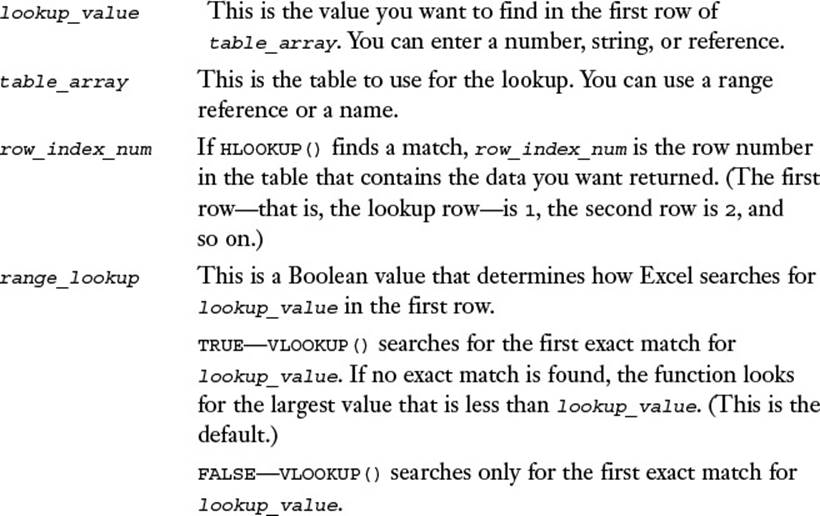
HLOOKUP(lookup_value, table_array, row_index_num[, range_lookup])
Returning a Customer Discount Rate with a Range Lookup
The most common use for VLOOKUP() and HLOOKUP() is to look for a match that falls within a range of values. This section and the next one take you through a few of examples of this range-lookup technique.
In business-to-business transactions, the cost of an item is often calculated as a percentage of the retail price. For example, a publisher might sell books to a bookstore at half the suggested list price. The percentage that the seller takes off the list price for the buyer is called the discount. Often, the size of the discount depends on the number of units ordered. For example, ordering 1-3 items might result in a 20% discount, ordering 4-24 items might result in a 40% discount, and so on.
Figure 9.3 shows a worksheet that uses VLOOKUP() to determine the discount a customer gets on an order, based on the number of units purchased.
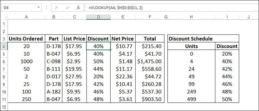
Figure 9.3 A worksheet that uses VLOOKUP() to look up a customer’s discount in a discount schedule.
For example, cell D4 uses the following formula:
=VLOOKUP(A4, $H$5:$I$11, 2)
The range_lookup argument is omitted, which means VLOOKUP() searches for the largest value that is less than or equal to the lookup value; in this case, this is the value in cell A4. Cell A4 contains the number of units purchased (20, in this case), and the range $H$5:$I$11 is the discount schedule table. VLOOKUP() searches down the first column (H5:H11) for the largest value that is less than or equal to 20. The first such cell is H6, because the value in H7 (24) is larger than 20. VLOOKUP() therefore moves to the second column (because you specifiedcol_index_num to be 2) of the table (cell I6) and grabs the value there (40%).
Tip
As I mentioned earlier in this section, both VLOOKUP() and HLOOKUP() return #N/A if no match is found in the lookup range. If you would prefer to return a friendlier or more useful message, use the IFNA() function to test whether the lookup will fail. Here’s the general idea:
=IFNA(LookupExpression, "LookupValue not found")
Here, LookupExpression is the VLOOKUP() or HLOOKUP() function, and LookupValue is the same as the lookup_value argument used in VLOOKUP() or HLOOKUP(). If IFNA() detects an #N/A error, the formula returns the "LookupValue not found"string; otherwise, it runs the lookup normally.
Returning a Tax Rate with a Range Lookup
Tax rates are perfect candidates for a range lookup because a given rate always applies to any income that is greater than some minimum amount and less than or equal to some maximum amount. For example, a rate of 25% might be applied to annual incomes over $37,450 and less than or equal to $90,750. Figure 9.4 shows a worksheet that uses VLOOKUP() to return the marginal tax rate, given a specified income.
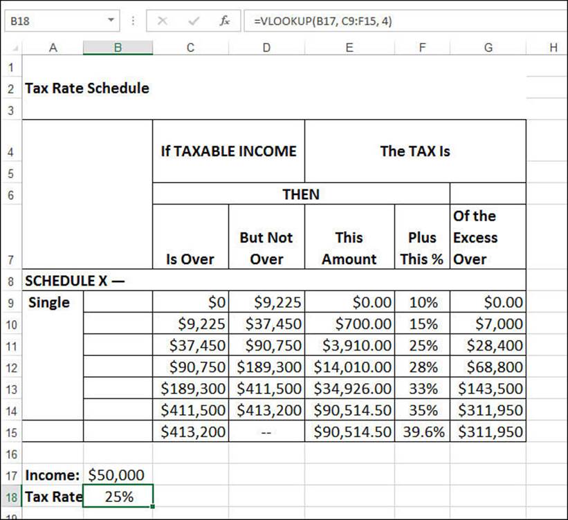
Figure 9.4 A worksheet that uses VLOOKUP() to look up a marginal income tax rate.
The lookup table is C9:F15, and the lookup value is cell B17, which contains the annual income. VLOOKUP() finds in column C the largest income that is less than or equal to the value in B17, which is $50,000. In this case, the matching value is $37,450 in cell C11. VLOOKUP() then looks in the fourth column to get the marginal rate in column F, which, in this case, is 25%.
Tip
You might find that you have multiple lookup tables in your model. For example, you might have multiple tax rate tables that apply to different types of taxpayers (single versus married, for example). If the tables use the same structure, you can use the IF() function to choose which lookup table is used in a lookup formula. Here’s the general formula:
=VLOOKUP(lookup_value, IF(condition, table1, table2), col_index_num)
If condition returns TRUE, a reference to table1 is returned, and that table is used as the lookup table; otherwise, table2 is used.
Finding Exact Matches
In many situations, a range lookup isn’t what you want. This is particularly true in lookup tables that contain a set of unique lookup values that represent discrete values instead of ranges. For example, if you need to look up a customer account number, a part code, or an employee ID, you want to be sure that your formula matches the value exactly. You can perform exact-match lookups with VLOOKUP() and HLOOKUP() by including the range_lookup argument with the value FALSE. The next couple sections demonstrate this technique.
Looking Up a Customer Account Number
A table of customer account numbers and names is a good example of a lookup table that contains discrete lookup values. In such a case, you want to use VLOOKUP() or HLOOKUP() to find an exact match for an account number you specify and then return the corresponding account name.Figure 9.5 shows a simple data-entry screen that automatically adds a customer name after the user enters the account number in cell B2.
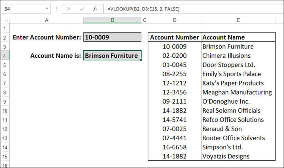
Figure 9.5 A simple data-entry worksheet that uses the exact-match version of VLOOKUP() to look up a customer’s name based on the entered account number.
The function that accomplishes this is in cell B4:
=VLOOKUP(B2, D3:E15, 2, FALSE)
The value in B2 is looked up in column D, and because the range_lookup argument is set to FALSE, VLOOKUP() searches for an exact match. If it finds one, it returns the text from column E.
Combining Exact-Match Lookups with In-Cell Drop-Down Lists
In Chapter 4, you learned how to use data validation to set up an in-cell drop-down list. Whatever value the user selects from the list is the value that’s stored in the cell. This technique becomes even more powerful when you combine it with exact-match lookups that use the current list selection as the lookup value.
![]() To learn how to use data validation to set up an in-cell drop-down list, see “Applying Data-Validation Rules to Cells,” p. 100.
To learn how to use data validation to set up an in-cell drop-down list, see “Applying Data-Validation Rules to Cells,” p. 100.
Figure 9.6 shows an example. Cell C9 contains a drop-down list that uses as its source the header values in row 1 (C1:N1). The formula in cell C10 uses HLOOKUP() to perform an exact-match lookup using the currently selected list value from C9:
=HLOOKUP(C9, C1:N7, 7, FALSE)
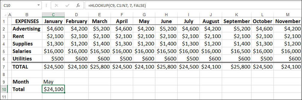
Figure 9.6 An HLOOKUP() formula in C10 performs an exact-match lookup in row 1 based on the current selection in C9’s in-cell drop-down list.
Advanced Lookup Operations
The basic lookup procedure—looking up a value in a column or row and then returning an offset value—will satisfy most of your needs. However, a few operations require a more sophisticated approach. The rest of this chapter examines these more advanced lookups, most of which make use of two more lookup functions: MATCH() and INDEX().
The MATCH() and INDEX() Functions
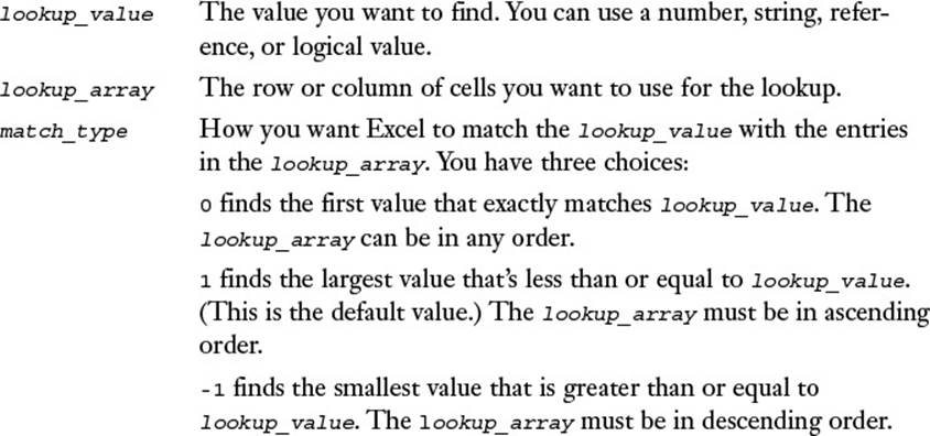
The MATCH() function looks through a row or column of cells for a value. If MATCH() finds a match, it returns the relative position of the match in the row or column. Here’s the syntax:
MATCH(lookup_value, lookup_array[, match_type])
Tip
You can use the usual wildcard characters within the lookup_value argument (provided that match_type is 0 and lookup_value is text). You can use the question mark (?) for single characters and the asterisk (*) for multiple characters.
Normally, you don’t use the MATCH() function by itself; you combine it with the INDEX() function. INDEX() returns the value of a cell at the intersection of a row and column inside a reference. Here’s the syntax for INDEX():
INDEX(reference, row_num[, column_num][, area_num])
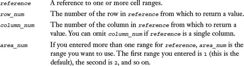
The idea is that you use MATCH() to get row_num or column_num (depending on how your table is laid out) and then use INDEX() to return the value you need.
To give you the flavor of using these two functions, let’s duplicate our earlier effort of looking up a customer name, given the account number. Figure 9.7 shows the result.
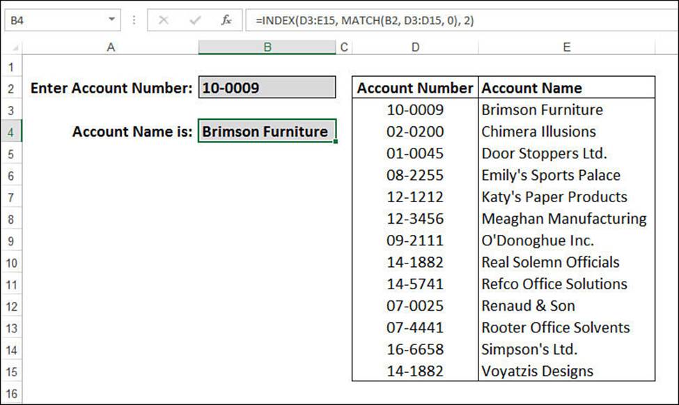
Figure 9.7 A worksheet that uses INDEX() and MATCH() to look up a customer’s name, based on the entered account number.
In particular, notice the new formula in cell B4:
=INDEX(D3:E15, MATCH(B2, D3:D15, 0), 2)
The MATCH() function looks up the value in cell B2 in the range D3:D15. That value is then used as the row_num argument for the INDEX() function. That value is 1 in the example, so the INDEX() function reduces to this:
=INDEX(D3:E15, 1, 2)
This returns the value in the first row and the second column of the range D3:E15.
Looking Up a Value Using Worksheet List Boxes
If you use a worksheet list box or combo box as explained in Chapter 4, the linked cell contains the number of the selected item, not the item itself. Figure 9.8 shows a worksheet with a list box and a drop-down list. The list used by both controls is the range A3:A10. Notice that the linked cells (E3 and E10) display the number of the list selection, not the selection itself.
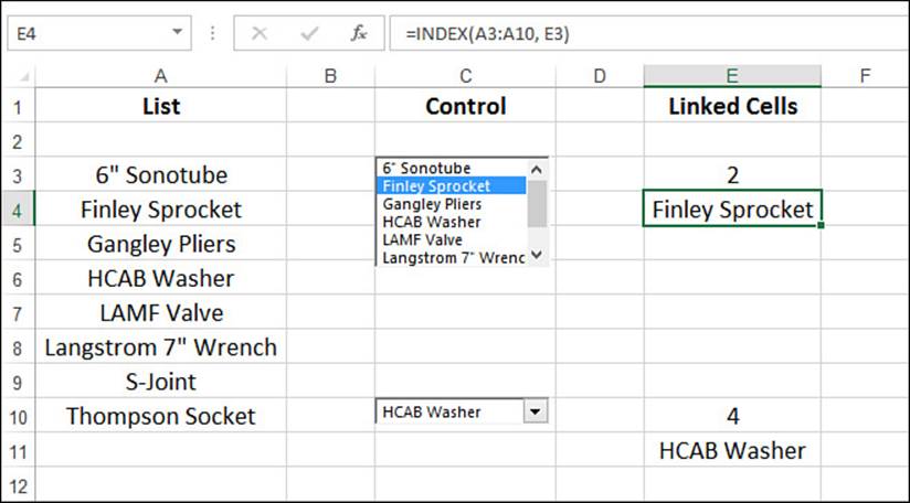
Figure 9.8 This worksheet uses INDEX() to get the selected item from a list box and a combo box.
To get the selected list item, you can use the INDEX() function with the following modified syntax:
INDEX(list_range, listelection)

For example, to find the item selected from the list box in Figure 9.8, you use the following formula:
=INDEX(A3:A10, E3)
Using Any Column as the Lookup Column
One of the major disadvantages of the VLOOKUP() function is that you must use the table’s leftmost column as the lookup column. (HLOOKUP() suffers from a similar problem: It must use the table’s topmost row as the lookup row.) This isn’t a problem if you remember to structure your lookup table accordingly, but that might not be possible in some cases, particularly if you inherit the data from someone else.
Fortunately, you can use the MATCH() and INDEX() combination to use any table column as the lookup column. For example, consider the parts database shown in Figure 9.9.
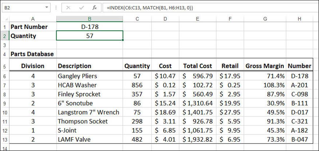
Figure 9.9 In this lookup table, the lookup values are in column H, and the value you want to find is in column C.
Column H contains the unique part numbers, so that’s what you want to use as the lookup column. The data you need is the quantity in column C. To accomplish this, you first find the part number (as given by the value in B1) in column H using MATCH():
MATCH(B1, H6:H13, 0)
When you know which row contains the part, you plug this result into an INDEX() function that operates only on the column that contains the data you want (column C):
=INDEX(C6:C13, MATCH(B1, H6:H13, 0))
Creating Row-and-Column Lookups
So far, all the lookups you’ve seen have been one dimensional, meaning that they searched for a lookup value in a single column or row. However, in many situations, you need a two-dimensional approach. This means that you need to look up a value in a column and a value in a row and then return the data value at the intersection of the two. I call this a row-and-column lookup.
You do this by using two MATCH() functions: one to calculate the INDEX() function’s row_num argument, and the other to calculate the INDEX() function’s column_num argument. Figure 9.10 shows an example.
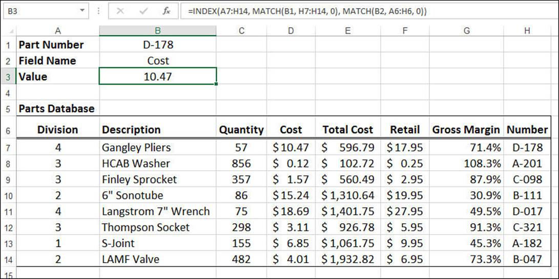
Figure 9.10 To perform a two-dimensional row-and-column lookup, use MATCH() functions to calculate both the row and the column values for the INDEX() function.
The idea here is to use both the part numbers (column H) and the field names (row 6) to return specific values from the parts database.
The part number is entered into cell B1, and getting the corresponding row in the parts table is no different from what you did in the previous section:
MATCH(B1, H7:H14, 0)
The field name is entered into cell B2. Getting the corresponding column number requires the following MATCH() expression:
MATCH(B2, A6:H6, 0)
These provide the INDEX() function’s row_num and column_num arguments (see cell B3):
=INDEX(A7:H14, MATCH(B1, H7:H14, 0), MATCH(B2, A6:H6, 0))
Creating Multiple-Column Lookups
Sometimes it’s not enough to look up a value in a single column. For example, in a list of employee names, you might need to look up both the first name and the last name if they’re in separate fields. One way to handle this is to create a new field that concatenates all the lookup values into a single item. However, it’s possible to do this without going to the trouble of creating a new concatenated field.
The secret is to perform the concatenation within the MATCH() function, as in this generic expression:
MATCH(value1 & value2, array1 & array2, match_type)
Here, value1 and value2 are the lookup values you want to work with, and array1 and array2 are the lookup columns. You can then plug the results into an array formula that uses INDEX() to get the needed data:
{=INDEX(reference, MATCH(value1 & value2, array1 & array2, match_type))}
For example, Figure 9.11 shows a database of employees, with separate fields for the first name, last name, title, and more.
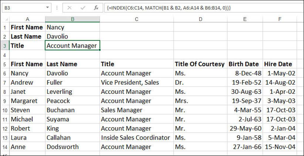
Figure 9.11 To perform a two-column lookup, use MATCH() to find a row based on the concatenated values of two or more columns.
The lookup values are in B1 (first name) and B2 (last name), and the lookup columns are A6:A14 (the First Name field) and B6:B14 (the Last Name field). Here’s the MATCH() function that looks up the required column:
MATCH(B1 & B2, A6:A14 & B6:B14, 0)
We want the specified employee’s title, so the INDEX() function looks in C6:C14 (the Title field). Here’s the array formula in cell B3:
{=INDEX(C6:C14, MATCH(B1 & B2, A6:A14 & B6:B14, 0))}
From Here
![]() To learn how to use data validation to set up an in-cell drop-down list, see “Applying Data-Validation Rules to Cells,” p. 100.
To learn how to use data validation to set up an in-cell drop-down list, see “Applying Data-Validation Rules to Cells,” p. 100.
![]() For the specifics of adding option buttons and list boxes to a worksheet, see “Understanding the Worksheet Controls,” p. 105.
For the specifics of adding option buttons and list boxes to a worksheet, see “Understanding the Worksheet Controls,” p. 105.
![]() For a general discussion of function syntax, see “The Structure of a Function,” p. 130.
For a general discussion of function syntax, see “The Structure of a Function,” p. 130.
![]() To learn about the WEEKDAY() function, see “The WEEKDAY() Function,” p. 214.
To learn about the WEEKDAY() function, see “The WEEKDAY() Function,” p. 214.
All materials on the site are licensed Creative Commons Attribution-Sharealike 3.0 Unported CC BY-SA 3.0 & GNU Free Documentation License (GFDL)
If you are the copyright holder of any material contained on our site and intend to remove it, please contact our site administrator for approval.
© 2016-2026 All site design rights belong to S.Y.A.