Microsoft Excel 2016 Step by Step (2015)
Part 1: Create and format workbooks
2. Work with data and Excel tables
In this chapter
![]() Enter and revise data
Enter and revise data
![]() Manage data by using Flash Fill
Manage data by using Flash Fill
![]() Move data within a workbook
Move data within a workbook
![]() Find and replace data
Find and replace data
![]() Correct and expand upon data
Correct and expand upon data
![]() Define Excel tables
Define Excel tables
Practice files
For this chapter, use the practice files from the Excel2016SBS\Ch02 folder. For practice file download instructions, see the introduction.
With Excel 2016, you can visualize and present information effectively by using charts, graphics, and formatting, but the data is the most important part of any workbook. By learning to enter data efficiently, you will make fewer data entry errors and give yourself more time to analyze your data so you can make decisions about your organization’s performance and direction.
Excel provides a wide variety of tools you can use to enter and manage worksheet data effectively. For example, you can organize your data into Excel tables so that you can store and analyze your data quickly and efficiently. Also, you can enter a data series quickly; repeat one or more values; and control how Excel formats cells, columns, and rows that you move from one part of a worksheet to another; all with a minimum of effort. With Excel, you can check the spelling of worksheet text, look up alternative words by using the thesaurus, and translate words to foreign languages.
This chapter guides you through procedures related to entering and revising Excel data, moving data within a workbook, finding and replacing existing data, using proofing and reference tools to enhance your data, and organizing your data by using Excel tables.
Enter and revise data
After you create a workbook, you can begin entering data. The simplest way to enter data is to click a cell and type a value. This method works very well when you’re entering a few pieces of data, but it is less than ideal when you’re entering long sequences or series of values. For example, you could create a worksheet tracking each customer’s monthly program savings.
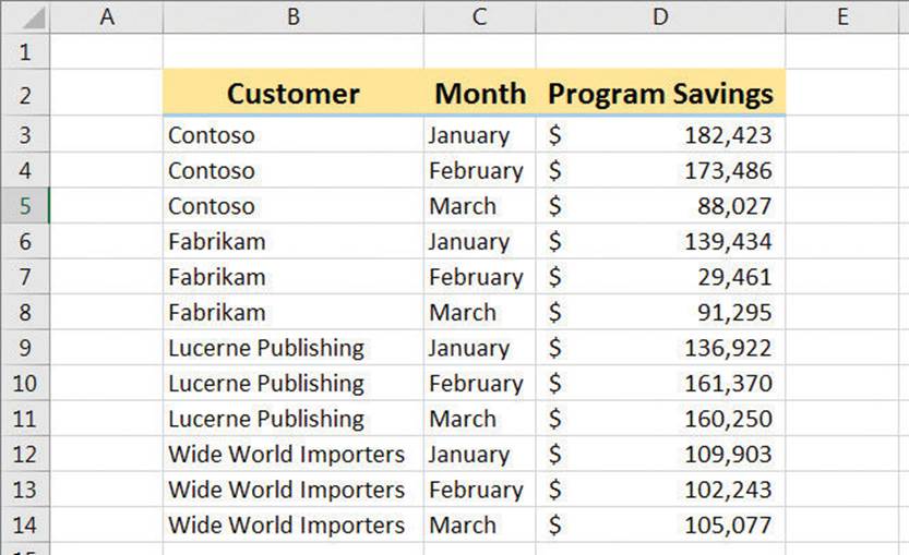
Store important business data in your worksheets
![]() Tip
Tip
To cancel data entry and return a cell to its previous state, press Esc.
Repeatedly entering the sequence January, February, March, and so on can be handled by copying and pasting the first occurrence of the sequence, but there’s an easier way to do it: use AutoFill. With AutoFill, you enter the first element in a recognized series, and then drag the fill handle in the lower-right corner of the cell until the series extends far enough to accommodate your data. By using a similar tool, FillSeries, you can enter two values in a series and use the fill handle to extend the series in your worksheet.
You do have some control over how Excel extends the values in a series when you drag the fill handle. If you drag the fill handle up (or to the left), Excel extends the series to include previous values. For example, if you enter January in a cell and then drag that cell’s fill handle up (or to the left), Excel places December in the first cell, November in the second cell, and so on.
Another way to control how Excel extends a data series is by holding down the Ctrl key while you drag the fill handle. If you select a cell that contains the value January and then drag the fill handle down, Excel extends the series by placing February in the next cell, March in the cell after that, and so on. If you hold down the Ctrl key while you drag the fill handle, however, Excel repeats the value January in each cell you add to the series.
![]() Tip
Tip
Experiment with how the fill handle extends your series and how pressing the Ctrl key changes that behavior. Using the fill handle can save you a lot of time entering data.
Other data entry techniques you’ll learn about in this topic are AutoComplete, which detects when a value you’re entering is similar to previously entered values; Pick From Drop-Down List, which you can use to choose a value from among the existing values in a column; and Ctrl+Enter, which you can use to enter a value in multiple cells simultaneously.
![]() Tip
Tip
If an AutoComplete suggestion doesn’t appear as you begin entering a cell value, the option might be turned off. To turn on AutoComplete, display the Backstage view, and then click Options. In the Excel Options dialog box, display the Advanced page. In the Editing Options section, select the Enable AutoComplete For Cell Values check box, and then click OK.
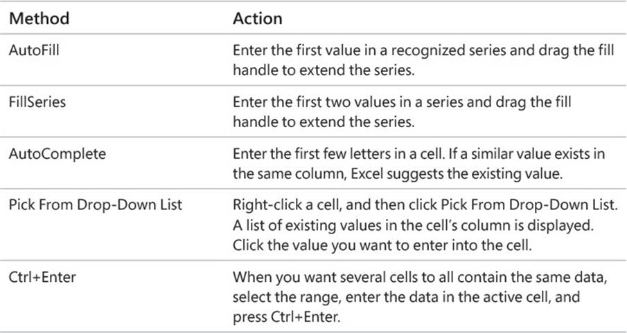
The following table summarizes these data entry techniques.
Another handy feature in Excel is the AutoFill Options button that appears next to data you add to a worksheet by using the fill handle.
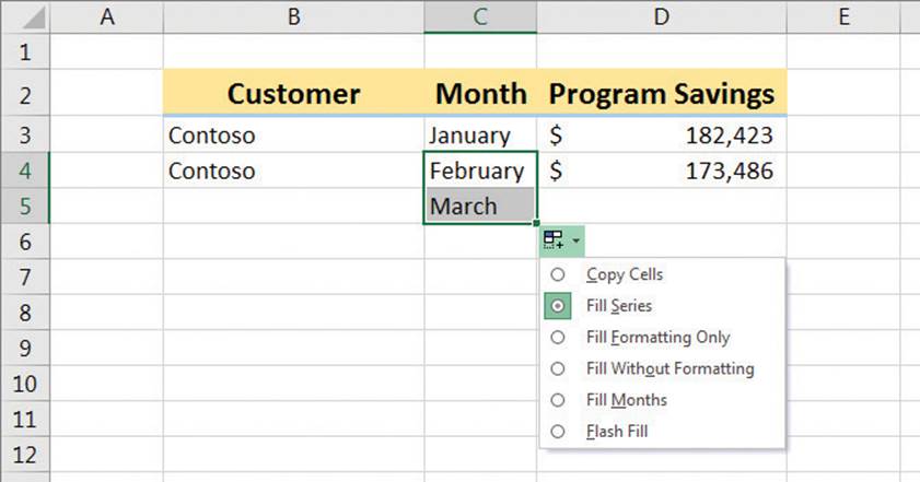
Use AutoFill options to control how the fill handle affects your data
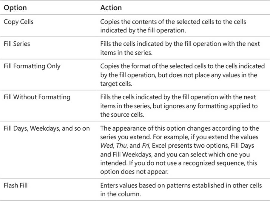
Clicking the AutoFill Options button displays a menu of actions Excel can take regarding the cells affected by your fill operation. The options on the menu are summarized in the following table.
![]() See Also
See Also
For more information about Flash Fill, see “Manage data by using Flash Fill” later in this chapter.
To enter values into a cell
1. Click the cell into which you want to enter the value.
2. Type the value by using the keyboard.
3. Press Enter to enter the value and move one cell down.
Or
Press Tab to enter the value and move one cell to the right.
To extend a series of values by using the fill handle
1. Select the cells that contain the series values.
2. Drag the fill handle to cover the cells where you want the new values to appear.
To enter a value into multiple cells at the same time
1. Select the cells into which you want to enter the value.
2. Enter the value.
3. Press Ctrl+Enter.
To enter cell data by using AutoComplete
1. Start entering a value into a cell.
2. Use the arrow keys or the mouse to highlight a suggested AutoComplete value.
3. Press Tab.
To enter cell data by picking from a list
1. Right-click the cell below a list of data.
2. Click Pick From Drop-down List.
3. Click the value you want to enter.
To control AutoFill options
1. Create an AutoFill sequence.
2. Click the AutoFill options button.
3. Click the option you want to apply.
Manage data by using Flash Fill
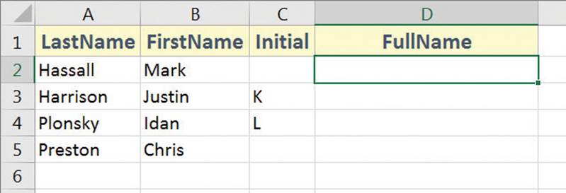
When you manage data in Excel, you will often find that you want to combine values from several cells into a single value. One common data configuration is to have a customer’s first name and last name in separate cells.
Fill in data according to a pattern by using Flash Fill
In this example, the contacts’ names appear in three columns: LastName, FirstName, and Initial. Note that not every contact has a middle initial. You could combine the names manually or by creating a formula, but Flash Fill can figure out the pattern if you give it a few examples.
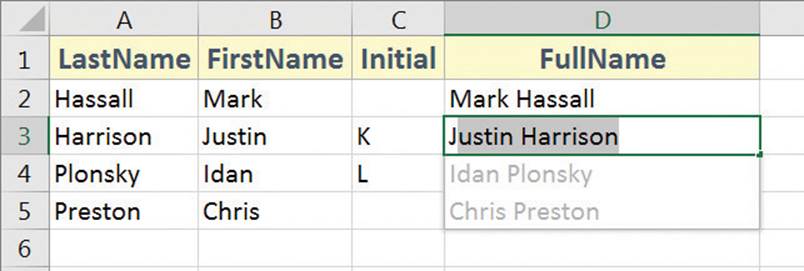
Flash Fill suggests values if it detects a pattern in your data
Note that Flash Fill did not include the middle initials in any row due to the lack of an initial in some of the rows. If you click in the FullName cell next to a row that contains an Initial value and edit the name as you would like it to appear, Flash Fill recognizes the new pattern for this subset of the data and offers to fill in the values. You can press Enter to accept the values Flash Fill suggests.
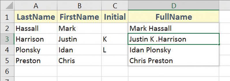
Edit a Flash Fill value to add data to the pattern
Flash Fill also lets you fix errors in your data. One common issue occurs when you try to enter numbers with leading zeros, such as United States postal codes, into cells formatted as General or with a number format. If you enter a zero-leading number into such a cell, Excel removes the zero.
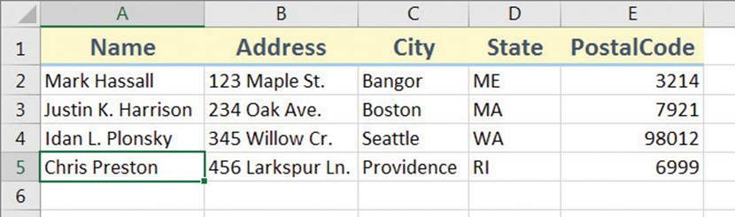
Use Flash Fill to correct common data-entry issues
To fix this error, you would select the cells that contain the postal codes and format the cells as text. Then, in the blank cell next to the first postal code that should have a leading zero, enter the postal code as it should appear, and press Enter. When you start entering the postal code into the second cell, Flash Fill offers to change the data by adding a zero to every value in the list.
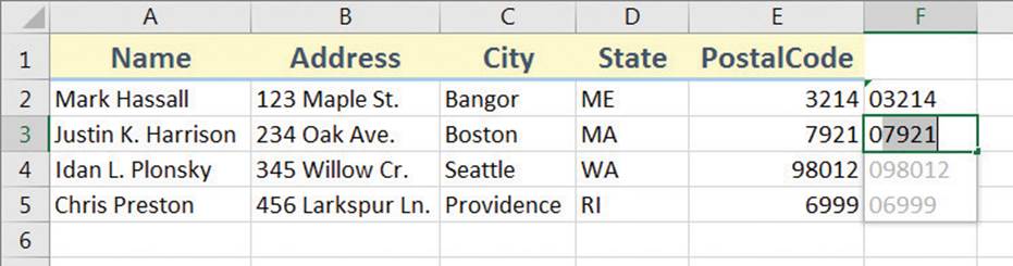
Flash Fill can overgeneralize the rule it applies to your data
The logic behind Flash Fill guessed that you wanted to add a zero to every postal code, but this change is incorrect for any value that should start with a number other than zero. To correct this, after you accept the values Flash Fill suggests, you would move to a blank cell next to a postal code that shouldn’t start with a zero and enter the correct value. When you do, Flash Fill updates its logic to suggest the correct values.
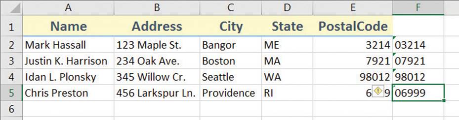
Correct Flash Fill changes to fix your data
![]() Tip
Tip
The error icon indicates that you have stored a number as text. Because you won’t be performing any mathematical operations on the postal code numbers, you can ignore the error.
To enter data by using Flash Fill
1. In a cell on the same row as data that can be combined or split, enter the result you want for that row’s data, and press Enter.
2. In the cell directly below the first cell into which you entered data, start entering a new value for the row.
3. Press Enter to accept the suggested values.
To correct a Flash Fill entry
1. Create a series of Flash Fill values in a worksheet.
2. Edit a cell that contains an incorrect Flash Fill value that so it contains the correct value.
3. Press Enter.
Move data within a workbook
You can move to a specific cell in lots of ways, but the most direct method is to start by clicking the cell with the contents you want to move. The cell you click will be outlined in black, and its contents, if any, will appear in the formula bar. When a cell is outlined, it is the active cell, meaning that you can modify its contents. You use a similar method to select multiple cells (referred to as a cell range). After you select the cell or cells you want to work with, you can cut, copy, delete, or change the format of the contents of the cell or cells.
![]() Important
Important
When you select a group of cells, the first cell you click is designated as the active cell.
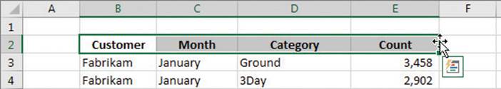
You’re not limited to selecting cells individually or as part of a range. For example, you might need to move a column of price data one column to the right to make room for a column of headings that indicate to which category a set of numbers belongs. To move an entire column (or entire columns) of data at a time, you click the column’s header, located at the top of the worksheet. Clicking a column header highlights every cell in that column so that you can copy or cut the column and paste it elsewhere in the workbook. Similarly, clicking a row’s header highlights every cell in that row, so that you can copy or cut the row and paste it elsewhere in the workbook.
When you copy a cell, cell range, row, or column, Excel copies the cells’ contents and formatting. The Paste Live Preview capability in Excel displays what your pasted data will look like without forcing you to commit to the paste operation.
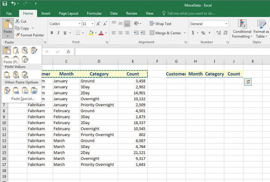
View live previews of your pasted data
If you point to one icon in the Paste gallery and then point to another icon without clicking, Excel will update the preview to reflect the new option. Depending on the cells’ contents, two or more of the paste options might lead to the same result.
![]() Tip
Tip
If pointing to an icon in the Paste gallery doesn’t result in a live preview, that option might be turned off. To turn Paste Live Preview on, in the Backstage view, click Options to open the Excel Options dialog box. Click General, select the Enable Live Preview check box, and click OK.
After you click an icon to complete the paste operation, Excel displays the Paste Options button next to the pasted cells. Clicking the Paste Options button also displays the Paste Options palette, but pointing to one of those icons doesn’t generate a preview. If you want to display Paste Live Preview again, you will need to press Ctrl+Z to undo the paste operation and, if necessary, cut or copy the data again to use the icons in the Clipboard group of the Home tab.
![]() Tip
Tip
If the Paste Options button doesn’t appear, you can turn the feature on by clicking Options in the Backstage view to open the Excel Options dialog box. In the Excel Options dialog box, display the Advanced page and then, in the Cut, Copy, And Paste area, select the Show Paste Options Button When Content Is Pasted check box. Click OK to close the dialog box and save your setting.
After cutting or copying data to the Clipboard, you can access additional paste options from the Paste gallery and from the Paste Special dialog box.
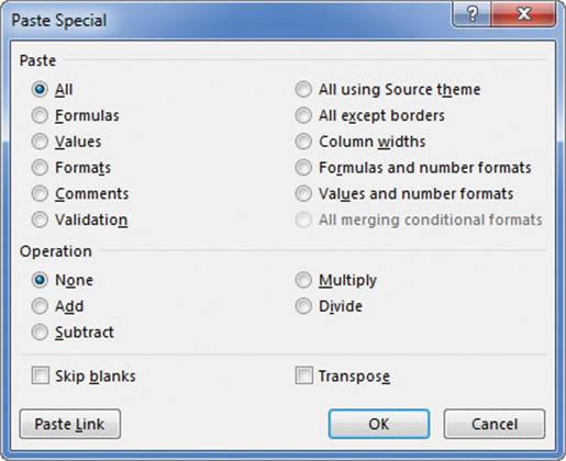
Use the Paste Special dialog box for uncommon paste operations
In the Paste Special dialog box, you can specify the aspect of the Clipboard contents you want to paste, restricting the pasted data to values, formats, comments, or one of several other options. You can perform mathematical operations involving the cut or copied data and the existing data in the cells you paste the content into, and you can transpose data—change rows to columns and columns to rows—when you paste it.
To select a cell or cell range
1. Click the first cell you want to select, and then drag to highlight the other cells you want to select.
To select disconnected groups of cells
1. Select a cell range.
2. Hold down the Ctrl key and select subsequent groups of cells.
To move a cell range
1. Select a cell range.
2. Point to the edge of the selection.
Move a cell range by dragging its border
3. Drag the range to its new location.
![]() Tip
Tip
If you move the cell range to cover cells that already contain values, Excel displays a message box asking if you want to replace the existing data.
To select one or more rows
1. Do any of the following:
• At the left edge of the worksheet, click the row’s header.
• Click a row header and drag to select other row headers.
• Click a row header, press and hold the Ctrl key, and click the headers of other rows you want to copy. The rows do not need to be adjacent to the first row.
To select one or more columns
1. Do any of the following:
• At the top edge of the worksheet, click the column’s header.
• Click a column header and drag to select other column headers.
• Click a column header, press and hold the Ctrl key, and click the column headers of other columns you want to copy. The columns do not need to be adjacent to the first column.
To copy a cell range
1. Select the cell range you want to copy.
2. On the Home tab of the ribbon, in the Clipboard group, click Copy.
Or
Press Ctrl+C.
To cut a cell range
1. Select the cell range you want to cut.
2. In the Clipboard group, click Cut.
Or
Press Ctrl+X.
To paste a cell range
1. Cut or copy a cell range.
2. Click the cell in the upper-left corner of the range where you want the pasted range to appear.
3. In the Clipboard group, click Paste.
Or
Press Ctrl+V.
To paste a cell range by using paste options
1. Copy a cell range.
2. Click the cell in the upper-left corner of the range where you want the pasted range to appear.
3. In the Clipboard group, click the Paste arrow (not the button).
4. Click the icon representing the paste operation you want to use.
To display a preview of a cell range you want to paste
1. Copy a cell range.
2. Click the cell in the upper-left corner of the range where you want the pasted range to appear.
3. Click the Paste arrow (not the button).
4. Point to the paste operation for which you want to see a preview.
To paste a cell range by using the Paste Special dialog box controls
1. Copy a cell range.
2. Click the cell in the upper-left corner of the range where you want the pasted range to appear.
3. Click the Paste arrow (not the button), and then click Paste Special.
4. Select the options you want for the paste operation.
5. Click OK.
Find and replace data
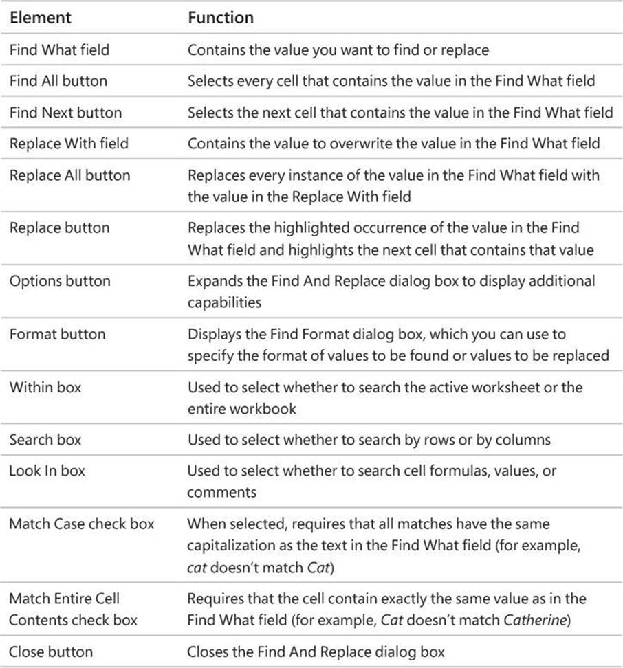
Excel worksheets can hold more than one million rows of data, so in large data collections it’s unlikely that you would have the time to move through a worksheet one row at a time to locate the data you want to find. You can locate specific data in an Excel worksheet by using the Find And Replace dialog box, which has two tabs (one named Find, the other named Replace) that you can use to search for cells that contain particular values. Using the controls on the Find tab identifies cells that contain the data you specify; by using the controls on the Replace tab, you can substitute one value for another.
![]() Tip
Tip
To display the Find tab of the Find And Replace dialog box by using a keyboard shortcut, press Ctrl+F. Press Ctrl+H to display the Replace tab of the Find And Replace dialog box.
When you need more control over the data that you find and replace—for instance, if you want to find cells in which the entire cell value matches the value you’re searching for—you can expand the Find And Replace dialog box to display more options.
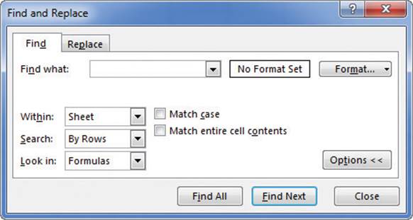
Expand the Find And Replace dialog box for more options
![]() Tip
Tip
By default, Excel looks in formulas, not cell values. To change that option, in the Look In drop-down list, click Values.
The following table summarizes the elements of the Find And Replace dialog box.
To edit a cell’s contents
1. Do any of the following:
• Click the cell, enter a new value, and press Enter.
• Click the cell, edit the value on the formula bar, and press Enter.
• Double-click the cell, edit the value in the body of the cell, and press Enter.
To edit part of a cell’s contents
1. Click the cell.
2. Edit the part of the cell’s value that you want to change on the formula bar.
3. Press Enter.
Or
1. Double-click the cell.
2. Edit the part of the cell’s value that you want to change in the body of the cell.
3. Press Enter.
To find the next occurrence of a value in a worksheet
1. On the Home tab, in the Editing group, click the Find & Select button to display a menu of choices, and then click Find.
2. In the Find what box, enter the value you want to find.
3. Click Find Next.
To find all instances of a value in a worksheet
1. On the Find & Select menu, click Find.
2. In the Find what box, enter the value you want to find.
3. Click Find All.
To replace a value with another value
1. On the Find & Select menu, click Replace.
2. In the Find what box, enter the value you want to change.
3. In the Replace with box, enter the value you want to replace the value from the Find what box.
4. Click the Replace button to replace the next occurrence of the value.
Or
Click the Replace All button to replace all occurrences of the value.
To require Find or Replace to match an entire cell’s contents
1. On the Find & Select menu, click either Find or Replace.
2. Set your Find or Replace values.
3. Click Options.
4. Select the Match entire cell contents check box.
5. Complete the find or replace operation.
To require Find or Replace to match cell contents, including uppercase and lowercase letters
1. On the Find & Select menu, click either Find or Replace.
2. Set your Find or Replace values.
3. Click Options.
4. Select the Match case check box.
5. Complete the find or replace operation.
To find or replace formats
1. On the Find & Select menu, click either Find or Replace.
2. Set your Find or Replace values.
3. Click Options.
4. Click the Find what row’s Format button, set a format by using the Find Format dialog box, and click OK.
5. If you want to perform a Replace operation, click the Replace with row’s Format button, set a format by using the Find Format dialog box, and click OK.
6. Finish your find or replace operation.
Correct and expand upon data
After you enter your data, you should take the time to check and correct it. You do need to verify visually that each piece of numeric data is correct, but you can make sure that your worksheet’s text is spelled correctly by using the Excel spelling checker. When the spelling checker encounters a word it doesn’t recognize, it highlights the word and offers suggestions representing its best guess of the correct word. You can then edit the word directly, pick the proper word from the list of suggestions, or have the spelling checker ignore the misspelling. You can also use the spelling checker to add new words to a custom dictionary so that Excel will recognize them later, saving you time by not requiring you to identify the words as correct every time they occur in your worksheets.
![]() Tip
Tip
To start checking spelling by using a keyboard shortcut, press F7.
After you make a change in a workbook, you can usually remove the change as long as you haven’t closed the workbook. You can even change your mind again if you decide you want to restore your change.
![]() Tip
Tip
To undo an action by using a keyboard shortcut, press Ctrl+Z. To redo an action, press Ctrl+Y.
Excel 2016 includes a new capability called Smart Lookup, which lets you find information relating to a highlighted word or phrase by using the Bing search engine. Excel displays the Insights task pane, which has two tabs: Explore and Define. The Explore tab displays search results from Wikipedia and other web resources. The Define tab displays definitions provided by OxfordDictionaries from Oxford University Press.
If you’re not sure of your word choice, or if you use a word that is almost but not quite right for your intended meaning, you can check for alternative words by using the thesaurus.
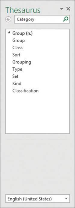
Get suggestions for alternative words by using the thesaurus
Finally, if you want to translate a word from one language to another, you can do so by selecting the cell that contains the value you want to translate and clicking the Translate button on the Review tab. The Research task pane opens (or changes if it’s already open) and displays tools you can use to select the original and destination languages.
![]() Important
Important
Excel displays a message box indicating that the information will be sent over the web to a third-party translation service. Click Yes to agree. If you don’t want Excel to display this message box in the future, select the Don’t Show Again check box and click Yes.
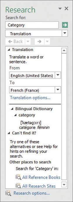
Translate words to other languages
![]() Important
Important
Excel translates a sentence by using word substitutions, which means that the translation routine doesn’t always pick the best word for a particular context. The translated sentence might not capture your exact meaning.
To undo or redo an action
1. Do either of the following:
• Click the Undo button on the Quick Access Toolbar to undo the action.
• Click the Redo button on the Quick Access Toolbar to restore the change.
To check spelling in a worksheet
1. Click Spelling.
2. For the first misspelled word, do one of the following:
• Click Change to accept the first suggested replacement for this occurrence of the word.
• Click a word from the Suggestions list and click Change.
• Enter the spelling you want in the Not in Dictionary box and click Change.
• Click Ignore Once to ignore this occurrence and move to the next misspelled word.
• Click Ignore All to ignore all occurrences of the word.
• Click the word with which you want to replace the misspelled word and click Change All.
3. Repeat step 2 until you have checked spelling for the entire worksheet.
4. Click Close.
![]() Tip
Tip
Excel starts checking spelling with the active cell. If that cell isn’t A1, Excel asks if you want to continue checking spelling from the beginning of the worksheet.
To add a word to the main dictionary
1. Click Spelling.
2. When the word you want to add appears in the Not in Dictionary box, click Add to Dictionary.
3. Finish checking spelling and click Close.
To change the dictionary used to check spelling
1. Click Spelling.
2. Click the the arrow next to the Dictionary language box, and click the dictionary you want to use.
To look up word alternatives by using the thesaurus
1. Select the cell that contains the word for which you want to find alternatives.
2. In the Proofing group, click Thesaurus.
3. Use the tools in the Thesaurus task pane to find alternative words.
4. On the title bar of the Thesaurus task pane, click the Close button to close the task pane.
To research a word by using Smart Lookup
1. Select the cell that contains the word you want to research.
2. In the Insights group, click the Smart Lookup button.
3. On the Explore tab of the Insights task pane, use the resources in the Explore with Wikipedia and other web resources lists.
Or
On the Define tab of the task pane, look up definitions of the selected word.
4. On the title bar of the Insights task pane, click the Close button to close the task pane.
To translate a word from one language to another
1. Click the cell that contains the word you want to translate.
2. In the Language group, click Translate.
3. If necessary, click Yes to send the text over the Internet.
4. Review the results.
5. Click the Close button to close the task pane.
Define Excel tables
With Excel, you’ve always been able to manage lists of data effectively, so that you can sort your worksheet data based on the values in one or more columns, limit the data displayed by using criteria (for example, show only those routes with fewer than 100 stops), and create formulas that summarize the values in visible (that is, unfiltered) cells. Excel 2016 provides those capabilities, and more, through Excel tables.
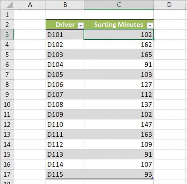
Manage data by using Excel tables
![]() Tip
Tip
Sorting, filtering, and summarizing data are all covered elsewhere in this book.
Excel can also create an Excel table from an existing cell range as long as the range has no blank rows or columns within the data and there is no extraneous data in cells immediately below or next to the list. If your existing data has formatting applied to it, that formatting remains applied to those cells when you create the Excel table, but you can have Excel replace the existing formatting with the Excel table’s formatting.
![]() Tip
Tip
To create an Excel table by using a keyboard shortcut, press Ctrl+L and then click OK.
Entering values into a cell below or to the right of an Excel table adds a row or column to the Excel table. After you enter the value and move out of the cell, the AutoCorrect Options action button appears. If you didn’t mean to include the data in the Excel table, you can click Undo Table AutoExpansion to exclude the cells from the Excel table. If you never want Excel to include adjacent data in an Excel table again, click Stop Automatically Expanding Tables.
![]() Tip
Tip
To stop Table AutoExpansion before it starts, click Options in the Backstage view. In the Excel Options dialog box, click Proofing, and then click the AutoCorrect Options button to open the AutoCorrect dialog box. Click the AutoFormat As You Type tab, clear the Include New Rows And Columns In Table check box, and then click OK twice.
You can resize an Excel table manually by using your mouse. If your Excel table’s headers contain a recognizable series of values (such as Region1, Region2, and Region3), and you drag the resize handle to create a fourth column, Excel creates the column with a label that is the next value in the series—in this example, Region4.
Excel tables often contain data you can summarize by calculating a sum or average, or by finding the maximum or minimum value in a column. To summarize one or more columns of data, you can add a total row to your Excel table.
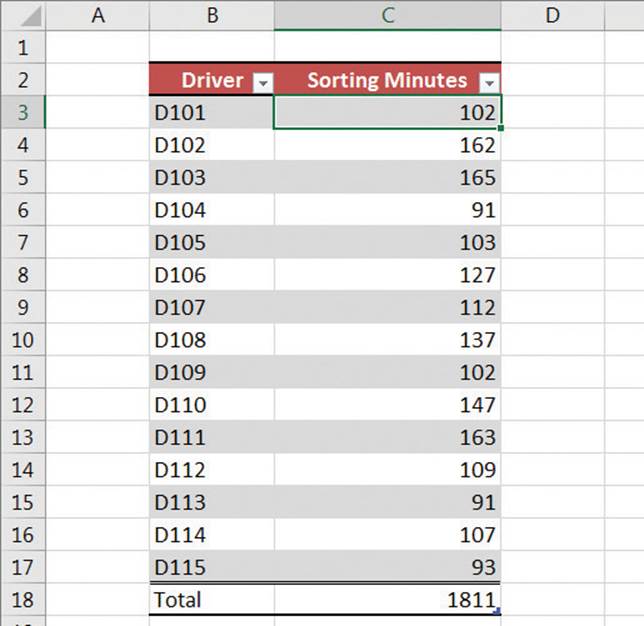
An Excel table with a total row
When you add the total row, Excel creates a formula that summarizes the values in the rightmost Excel table column. You can change the summary function by picking a new one from the partial list displayed in the Excel table or by selecting a function from the full set.
Much as it does when you create a new worksheet, Excel gives your Excel tables generic names such as Table1 and Table2. You can change an Excel table’s name to something easier to recognize in your formulas. Changing an Excel table name might not seem important, but it helps make formulas that summarize Excel table data much easier to understand. You should make a habit of renaming your Excel tables so you can recognize the data they contain.
![]() See Also
See Also
For more information about using the Insert Function dialog box and about referring to tables in formulas, see “Create formulas to calculate values” in Chapter 3, “Perform calculations on data.”
If for any reason you want to convert your Excel table back to a normal range of cells, you can do so quickly.
To create an Excel table
1. Click a cell in the list of data you want to make into an Excel table.
2. On the Home tab, in the Styles group, click Format as Table.
3. Click the style you want to apply to the table.
4. Verify that the cell range is correct.
5. If necessary, select or clear the My table has headers check box, and then click OK.
To create an Excel table with default formatting
1. Click a cell in the range that you want to make into an Excel table.
2. Press Ctrl+L.
3. Click OK.
To add a column or row to an Excel table
1. Click a cell in the row below or the column to the right of the Excel table.
2. Enter the data and press Enter.
To expand or contract an Excel table
1. Click any cell in the Excel table.
2. Point to the lower-right corner of the Excel table.
3. When the mouse pointer changes to a diagonal arrow, drag the Excel table’s outline to redefine the table.
To add a total row to an Excel table
1. Click any cell in the Excel table.
2. On the Design tool tab of the ribbon, in the Table Style Options group, select the Total Row check box.
To change the calculation used in a total row cell
1. Click any Total row cell that contains a calculation.
2. Click the cell’s arrow.
3. Select a summary function.
Or
Click More Functions, use the Insert Function dialog box to create the formula, and click OK.
To rename an Excel table
1. Click any cell in the Excel table.
2. On the Design tool tab, in the Properties group, enter a new name for the Excel table in the Table Name box.
3. Press Enter.
To convert an Excel table to a cell range
1. Click any cell in the Excel table.
2. On the Design tool tab, in the Tools group, click Convert to Range.
3. In the confirmation dialog box that appears, click Yes.
Skills review
In this chapter, you learned how to:
![]() Enter and revise data
Enter and revise data
![]() Manage data by using Flash Fill
Manage data by using Flash Fill
![]() Move data within a workbook
Move data within a workbook
![]() Find and replace data
Find and replace data
![]() Correct and expand upon data
Correct and expand upon data
![]() Define Excel tables
Define Excel tables
 Practice tasks
The practice files for these tasks are located in the Excel2016SBS\Ch02 folder. You can save the results of the tasks in the same folder.
Enter and revise data
Open the EnterData workbook in Excel, and then perform the following tasks:
1. Use the fill handle to copy the value from cell B3, Fabrikam, to cells B4:B7.
2. Extend the series of months starting in cell C3 to cell C7, and then use the Auto Fill Options button to copy the cell’s value instead of extending the series.
3. In cell B8, enter the letters Fa and accept the AutoComplete value Fabrikam.
4. In cell C8, enter February.
5. Enter the value Ground in cell D8 by using Pick From Drop-down List.
6. Edit the value in cell E5 to $6,591.30.
Manage data by using Flash Fill
Open the CompleteFlashFill workbook in Excel, and then perform the following tasks:
1. On the Names worksheet, in cell D2, enter Mark Hassall and press Enter.
2. In cell D3, enter J and, when Excel displays a series of names in column D, press Enter to accept the Flash Fill suggestions.
3. Edit the value in cell D3 to include the middle initial found in cell C3, and press Enter.
4. Click the Addresses sheet tab.
5. Select cells F2:F5 and then, on the Home tab, in the Number group, click the arrow next to the Number Format button and click Text.
6. In cell F2, enter 03214 and press Enter.
7. In cell F3, enter 0 and then press Enter to accept the Flash Fill suggestions.
8. Edit the value in cell F4 to read 98012.
Move data within a workbook
Open the MoveData workbook in Excel, and then perform the following tasks:
1. On the Count worksheet, copy the values in cells B2:D2.
2. Display the Sales worksheet, preview what the data would look like if pasted as values only, and paste the contents you just copied into cells B2:D2.
3. On the Sales worksheet, cut column I and paste it into the space currently occupied by column E.
Find and replace data
Open the FindValues workbook in Excel, and then perform the following tasks:
1. On the Time Summary worksheet, find the cell that contains the value 114.
2. On the Time Summary worksheet, find the cell with contents formatted as italic type.
3. Click the Customer Summary sheet tab.
4. Replace all instances of the value Contoso with the value Northwind Traders.
Correct and expand upon data
Open the ResearchItems workbook in Excel, and then perform the following tasks:
1. Check spelling in the file and accept the suggested changes for shipped and within.
2. Ignore the suggestion for TwoDay.
3. Add the word ThreeDay to the main dictionary.
4. Use the Thesaurus to find alternate words for the word Overnight in cell B6, then translate the same word to French.
5. Click cell B2 and use Smart Lookup to find more information about the word level.
Define Excel tables
Open the CreateExcelTables workbook in Excel, and then perform the following tasks:
1. Create an Excel table from the list of data on the Sort Times worksheet.
2. Add a row of data to the Excel table for driver D116, and assign a value of 100 sorting minutes.
3. Add a Total row to the Excel table, and then change the summary function to Average.
4. Rename the Excel table to SortTimes.
All materials on the site are licensed Creative Commons Attribution-Sharealike 3.0 Unported CC BY-SA 3.0 & GNU Free Documentation License (GFDL)
If you are the copyright holder of any material contained on our site and intend to remove it, please contact our site administrator for approval.
© 2016-2026 All site design rights belong to S.Y.A.