Microsoft Excel 2016 Step by Step (2015)
Part 1: Create and format workbooks
3. Perform calculations on data
In this chapter
![]() Name groups of data
Name groups of data
![]() Create formulas to calculate values
Create formulas to calculate values
![]() Summarize data that meets specific conditions
Summarize data that meets specific conditions
![]() Set iterative calculation options and enable or disable automatic calculation
Set iterative calculation options and enable or disable automatic calculation
![]() Use array formulas
Use array formulas
![]() Find and correct errors in calculations
Find and correct errors in calculations
Practice files
For this chapter, use the practice files from the Excel2016SBS\Ch03 folder. For practice file download instructions, see the introduction.
Excel 2016 workbooks give you a handy place to store and organize your data, but you can also do a lot more with your data in Excel. One important task you can perform is to calculate totals for the values in a series of related cells. You can also use Excel to discover other information about the data you select, such as the maximum or minimum value in a group of cells. Regardless of your needs, Excel gives you the ability to find the information you want. And if you make an error, you can find the cause and correct it quickly.
Often, you can’t access the information you want without referencing more than one cell, and it’s also often true that you’ll use the data in the same group of cells for more than one calculation. Excel makes it easy to reference several cells at the same time, so that you can define your calculations quickly.
This chapter guides you through procedures related to streamlining references to groups of data on your worksheets and creating and correcting formulas that summarize an organization’s business operations.
Name groups of data
When you work with large amounts of data, it’s often useful to identify groups of cells that contain related data. For example, you can create a worksheet in which columns of cells contain data summarizing the number of packages handled during a specific time period and each row represents a region.
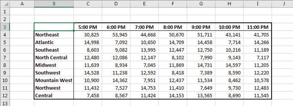
Worksheets often contain logical groups of data
Instead of specifying the cells individually every time you want to use the data they contain, you can define those cells as a range (also called a named range). For example, you can group the hourly packages handled in the Northeast region into a group called NortheastVolume. Whenever you want to use the contents of that range in a calculation, you can use the name of the range instead of specifying the range’s address.
![]() Tip
Tip
Yes, you could just name the range Northeast, but if you use the range’s values in a formula in another worksheet, the more descriptive range name tells you and your colleagues exactly what data is used in the calculation.
If the cells you want to define as a named range have labels in a row or column that’s part of the cell group, you can use those labels as the names of the named ranges. For example, if your data appears in worksheet cells B4:I12 and the values in column B are the row labels, you can make each row its own named range.
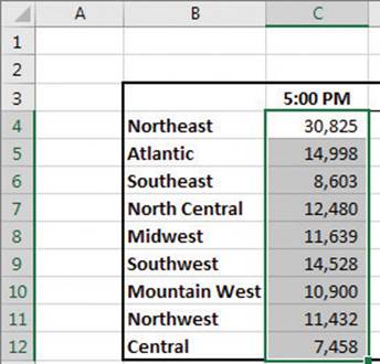
Select a group of cells to create a named range
If you want to manage the named ranges in your workbook, perhaps to edit a range’s settings or delete a range you no longer need, you can do so in the Name Manager dialog box.
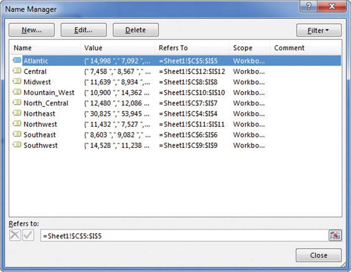
Manage named ranges in the Name Manager dialog box
![]() Tip
Tip
If your workbook contains a lot of named ranges, you can click the Filter button in the Name Manager dialog box and select a criterion to limit the names displayed in the dialog box.
To create a named range
1. Select the cells you want to include in the named range.
2. In the Name box, which is next to the formula bar, enter the name for your named range.
Or
1. Select the cells you want to include in the named range.
2. On the Formulas tab of the ribbon, in the Defined Names group, click Define Name.
3. In the New Name dialog box, enter a name for the named range.
4. Verify that the named range includes the cells you want.
5. Click OK.
To create a series of named ranges from worksheet data with headings
1. Select the cells that contain the headings and data cells you want to include in the named ranges.
2. In the Defined Names group, click Create from Selection.
3. In the Create Names from Selection dialog box, select the check box next to the location of the heading text from which you want to create the range names.
4. Click OK.
To edit a named range
1. In the Defined Names group, click Name Manager.
2. Click the named range you want to edit.
3. In the Refers to box, change the cells that the named range refers to.
Or
Click Edit, edit the named range in the Edit Range box, and click OK.
4. Click Close.
To delete a named range
1. Click Name Manager.
2. Click the named range you want to delete.
3. Click Delete.
4. Click Close.
Create formulas to calculate values
After you add your data to a worksheet and define ranges to simplify data references, you can create a formula, which is an expression that performs calculations on your data. For example, you can calculate the total cost of a customer’s shipments, figure the average number of packages for all Wednesdays in the month of January, or find the highest and lowest daily package volumes for a week, month, or year.
To write an Excel formula, you begin the cell’s contents with an equal (=) sign; Excel then knows that the expression following it should be interpreted as a calculation, not text. After the equal sign, you enter the formula. For example, you can find the sum of the numbers in cells C2 and C3 by using the formula =C2+C3. After you have entered a formula into a cell, you can revise it by clicking the cell and then editing the formula in the formula bar. For example, you can change the preceding formula to =C3-C2, which calculates the difference between the contents of cells C2 and C3.
![]() Important
Important
If Excel treats your formula as text, make sure that you haven’t accidentally put a space before the equal sign. Remember, the equal sign must be the first character!
Entering the cell references for 15 or 20 cells in a calculation would be tedious, but in Excel you can easily enter complex calculations by using the Insert Function dialog box. The Insert Function dialog box includes a list of functions, or predefined formulas, from which you can choose.
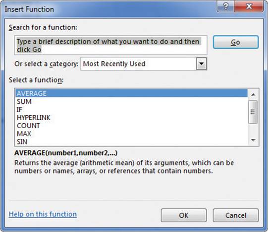
Create formulas with help in the Insert Function dialog box
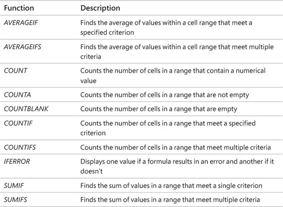
The following table describes some of the most useful functions in the list.
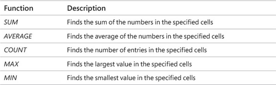
Two other functions you might use are the NOW and PMT functions. The NOW function displays the time at which Excel updated the workbook’s formulas, so the value will change every time the workbook recalculates. The proper form for this function is =NOW(). You could, for example, use the NOW function to calculate the elapsed time from when you started a process to the present time.
The PMT function is a bit more complex. It calculates payments due on a loan, assuming a constant interest rate and constant payments. To perform its calculations, the PMT function requires an interest rate, the number of payments, and the starting balance. The elements to be entered into the function are called arguments and must be entered in a certain order. That order is written as PMT(rate, nper, pv, fv, type). The following table summarizes the arguments in the PMT function.
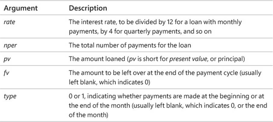
If a company wanted to borrow $2,000,000 at a 6 percent interest rate and pay the loan back over 24 months, you could use the PMT function to figure out the monthly payments. In this case, you would write the function =PMT(6%/12, 24, 2000000), which calculates a monthly payment of $88,641.22.
![]() Tip
Tip
The 6-percent interest rate is divided by 12 because the loan’s interest is compounded monthly.
You can also use the names of any ranges you defined to supply values for a formula. For example, if the named range NortheastLastDay refers to cells C4:I4, you can calculate the average of cells C4:I4 with the formula =AVERAGE(NortheastLastDay). With Excel, you can add functions, named ranges, and table references to your formulas more efficiently by using the Formula AutoComplete capability. Just as AutoComplete offers to fill in a cell’s text value when Excel recognizes that the value you’re typing matches a previous entry, Formula AutoComplete offers to help you fill in a function, named range, or table reference while you create a formula.
As an example, consider a worksheet that contains a two-column Excel table named Exceptions. The first column is labeled Route; the second is labeled Count.
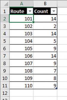
Excel tables track data in a structured format
You refer to a table by typing the table name, followed by the column or row name in brackets. For example, the table reference Exceptions[Count] would refer to the Count column in the Exceptions table.
To create a formula that finds the total number of exceptions by using the SUM function, you begin by typing =SU. When you enter the letter S, Formula AutoComplete lists functions that begin with the letter S; when you enter the letter U, Excel narrows the list down to the functions that start with the letters SU.
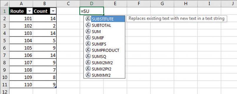
Excel displays Formula AutoComplete suggestions to help with formula creation
To add the SUM function (followed by an opening parenthesis) to the formula, click SUM and then press Tab. To begin adding the table reference, enter the letter E. Excel displays a list of available functions, tables, and named ranges that start with the letter E. Click Exceptions, and press Tab to add the table reference to the formula. Then, because you want to summarize the values in the table’s Count column, enter an opening bracket, and in the list of available table items, click Count. To finish creating the formula, enter a closing bracket followed by a closing parenthesis to create the formula =SUM(Exceptions[Count]).
If you want to include a series of contiguous cells in a formula, but you haven’t defined the cells as a named range, you can click the first cell in the range and drag to the last cell. If the cells aren’t contiguous, hold down the Ctrl key and select all of the cells to be included. In both cases, when you release the mouse button, the references of the cells you selected appear in the formula.
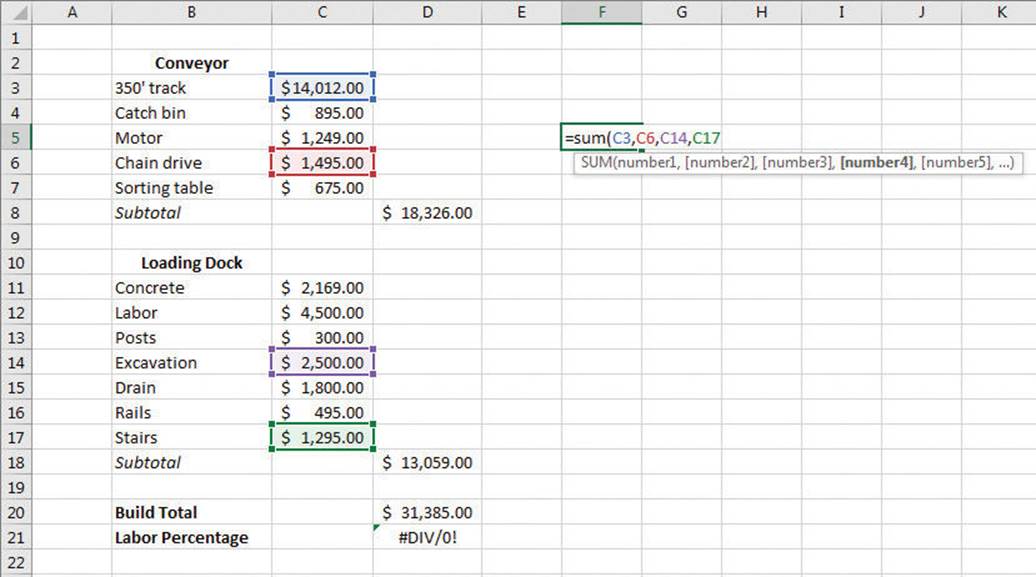
A SUM formula that adds individual cells instead of a continuous range
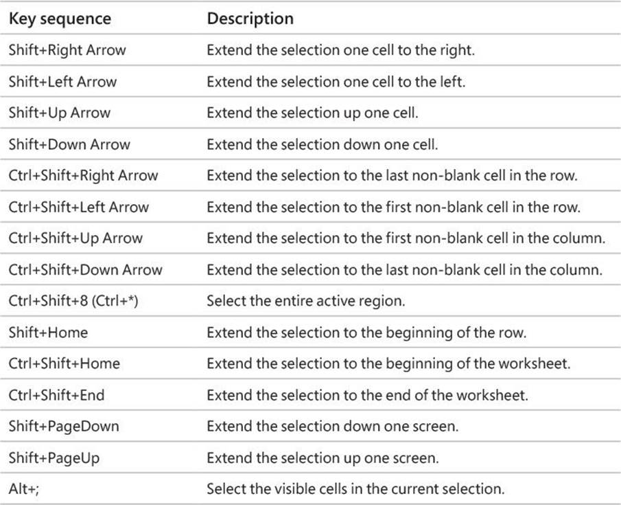
In addition to using the Ctrl key to add cells to a selection, you can expand a selection by using a wide range of keyboard shortcuts.
The following table summarizes many of those shortcuts.
After you create a formula, you can copy it and paste it into another cell. When you do, Excel tries to change the formula so that it works in the new cells. For instance, suppose you have a worksheet where cell D8 contains the formula =SUM(C2:C6). Clicking cell D8, copying the cell’s contents, and then pasting the result into cell D16 writes =SUM(C10:C14) into cell D16. Excel has reinterpreted the formula so that it fits the surrounding cells! Excel knows it can reinterpret the cells used in the formula because the formula uses a relative reference, or a reference that can change if the formula is copied to another cell. Relative references are written with just the cell row and column (for example, C14).
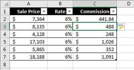
Relative references are useful when you summarize rows of data and want to use the same formula for each row. As an example, suppose you have a worksheet with two columns of data, labeled Sale Price and Rate, and you want to calculate your sales representative’s commission by multiplying the two values in a row. To calculate the commission for the first sale, you would enter the formula =A2*B2 in cell C2.
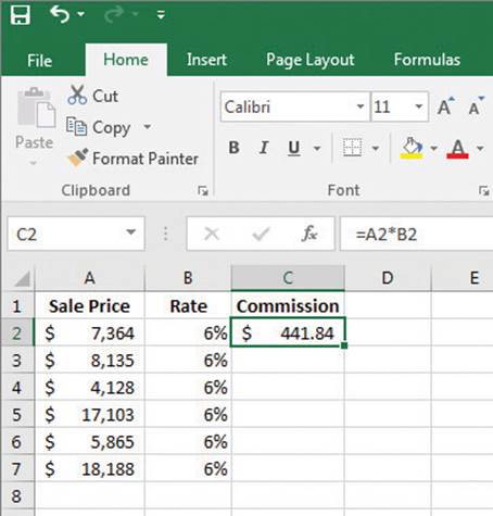
Use formulas to calculate values such as commissions
Selecting cell C2 and dragging the fill handle until it covers cells C2:C7 copies the formula from cell C2 into each of the other cells. Because you created the formula by using relative references, Excel updates each cell’s formula to reflect its position relative to the starting cell (in this case, cell C2.) The formula in cell C7, for example, is =A7*B7.
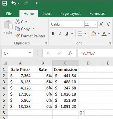
Copying formulas to other cells summarizes additional data
You can use a similar technique when you add a formula to an Excel table column. If the sale price and rate data were in an Excel table and you created the formula =A2*B2 in cell C2, Excel would apply the formula to every other cell in the column. Because you used relative references in the formula, the formulas would change to reflect each cell’s distance from the original cell.
Adding a formula to an Excel table cell creates a calculated column
If you want a cell reference to remain constant when you copy the formula that is using it to another cell, you can use an absolute reference. To write a cell reference as an absolute reference, you enter $ before the row letter and the column number. For example, if you want the formula in cell D16 to show the sum of values in cells C10 through C14 regardless of the cell into which it is pasted, you can write the formula as =SUM($C$10:$C$14).
![]() Tip
Tip
Another way to ensure that your cell references don’t change when you copy a formula to another cell is to click the cell that contains the formula, copy the formula’s text in the formula bar, press the Esc key to exit cut-and-copy mode, click the cell where you want to paste the formula, and press Ctrl+V. Excel doesn’t change the cell references when you copy your formula to another cell in this manner.
One quick way to change a cell reference from relative to absolute is to select the cell reference in the formula bar and then press F4. Pressing F4 cycles a cell reference through the four possible types of references:
![]() Relative columns and rows (for example, C4)
Relative columns and rows (for example, C4)
![]() Absolute columns and rows (for example, $C$4)
Absolute columns and rows (for example, $C$4)
![]() Relative columns and absolute rows (for example, C$4)
Relative columns and absolute rows (for example, C$4)
![]() Absolute columns and relative rows (for example, $C4)
Absolute columns and relative rows (for example, $C4)
To create a formula by entering it in a cell
1. Click the cell in which you want to create the formula.
2. Enter an equal sign (=).
3. Enter the remainder of the formula, and then press Enter.
To create a formula by using the Insert Function dialog box
1. On the Formulas tab, in the Function Library group, click the Insert Function button.
2. Click the function you want to use in your formula.
Or
Search for the function you want, and then click it.
3. Click OK.
4. In the Function Arguments dialog box, enter the function’s arguments.
5. Click OK.
To display the current date and time by using a formula
1. Click the cell in which you want to display the current date and time.
2. Enter =NOW() into the cell.
3. Press Enter.
To update a NOW() formula
1. Press F9.
To calculate a payment by using a formula
1. Create a formula with the syntax =PMT(rate, nper, pv, fv, type), where:
• rate is the interest rate, to be divided by 12 for a loan with monthly payments, by 4 for quarterly payments, and so on.
• nper is the total number of payments for the loan.
• pv is the amount loaned.
• fv is the amount to be left over at the end of the payment cycle.
• type is 0 or 1, indicating whether payments are made at the beginning or at the end of the month.
2. Press Enter.
To refer to a named range in a formula
1. Click the cell where you want to create the formula.
2. Enter = to start the formula.
3. Enter the name of the named range in the part of the formula where you want to use its values.
4. Complete the formula.
5. Press Enter.
To refer to an Excel table column in a formula
1. Click the cell where you want to create the formula.
2. Enter = to start the formula.
3. At the point in the formula where you want to include the table’s values, enter the name of the table.
Or
Use Formula AutoComplete to enter the table name.
4. Enter an opening bracket ([) followed by the column name.
Or
Enter [ and use Formula AutoComplete to enter the column name.
5. Enter ]) to close the table reference.
6. Press Enter.
To copy a formula without changing its cell references
1. Click the cell that contains the formula you want to copy.
2. Select the formula text in the formula bar.
3. Press Ctrl+C.
4. Click the cell where you want to paste the formula.
5. Press Ctrl+V.
6. Press Enter.
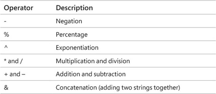
Operators and precedence
When you create an Excel formula, you use the built-in functions and arithmetic operators that define operations such as addition and multiplication. In Excel, mathematical operators are evaluated in the order listed in the following table.
If two operators at the same level, such as + and -, occur in the same equation, Excel evaluates them in left-to-right order. For example, the operations in the formula = 4 + 8 * 3 - 6 would be evaluated in this order:
1. 8 * 3, with a result of 24
2. 4 + 24, with a result of 28
3. 28 - 6, with a final result of 22
To move a formula without changing its cell references
1. Click the cell that contains the formula you want to copy.
2. Point to the edge of the cell you selected.
3. Drag the outline to the cell where you want to move the formula.
To copy a formula while changing its cell references
1. Click the cell that contains the formula you want to copy.
2. Press Ctrl+C.
3. Click the cell where you want to paste the formula.
4. Press Ctrl+V.
You can control the order in which Excel evaluates operations by using parentheses. Excel always evaluates operations in parentheses first. For example, if the previous equation were rewritten as = (4 + 8) * 3 - 6, the operations would be evaluated in this order:
1. (4 + 8), with a result of 12
2. 12 * 3, with a result of 36
3. 36 - 6, with a final result of 30
If you have multiple levels of parentheses, Excel evaluates the expressions within the innermost set of parentheses first and works its way out. As with operations on the same level, such as + and -, expressions in the same parenthetical level are evaluated in left-to-right order.
For example, the formula = 4 + (3 + 8 * (2 + 5)) - 7 would be evaluated in this order:
1. (2 + 5), with a result of 7
2. 7 * 8, with a result of 56
3. 56 + 3, with a result of 59
4. 4 + 59, with a result of 63
5. 63 - 7, with a final result of 56
To create relative and absolute cell references
1. Enter a cell reference into a formula.
2. Click within the cell reference.
3. Enter a $ in front of a row or column reference you want to make absolute.
Or
Press F4 to advance through the four possible combinations of relative and absolute row and column references.
Summarize data that meets specific conditions
Another use for formulas is to display messages when certain conditions are met. This kind of formula is called a conditional formula; one way to create a conditional formula in Excel is to use the IF function. Clicking the Insert Function button next to the formula bar and then choosing theIF function displays the Function Arguments dialog box with the fields required to create an IF formula.
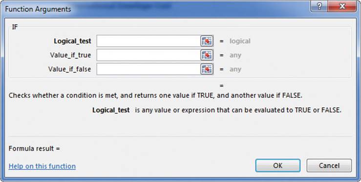
The Function Arguments dialog box for an IF formula
When you work with an IF function, the Function Arguments dialog box has three boxes: Logical_test, Value_if_true, and Value_if_false. The Logical_test box holds the condition you want to check.
Now you need to have Excel display messages that indicate whether the condition is met or not. To have Excel print a message from an IF function, you enclose the message in quotes in the Value_if_true or Value_if_false box. In this case, you would type “High-volume shipper—evaluate for rate decrease” in the Value_if_true box and “Does not qualify at this time” in the Value_if_false box.
Excel also includes several other conditional functions you can use to summarize your data, as shown in the following table.
You can use the IFERROR function to display a custom error message, instead of relying on the default Excel error messages to explain what happened. For example, you could use an IFERROR formula when looking up a value by using the VLOOKUP function. An example of creating this type of formula would be to look up a customer’s name, found in the second column of a table named Customers, based on the customer identification number entered into cell G8. That formula might look like this: =IFERROR(VLOOKUP(G8,Customers,2,false),”Customer not found”). If the function finds a match for the CustomerID in cell G8, it displays the customer’s name; if it doesn’t find a match, it displays the text Customer not found.
![]() Tip
Tip
The last two arguments in the VLOOKUP function tell the formula to look in the Customers table’s second column and to require an exact match. For more information about the VLOOKUP function, see “Look up information in a worksheet” in Chapter 6, “Reorder and summarize data.”
Just as the COUNTIF function counts the number of cells that meet a criterion and the SUMIF function finds the total of values in cells that meet a criterion, the AVERAGEIF function finds the average of values in cells that meet a criterion. To create a formula that uses the AVERAGEIFfunction, you define the range to be examined for the criterion, the criterion, and, if required, the range from which to draw the values. As an example, consider a worksheet that lists each customer’s ID number, name, state, and total monthly shipping bill.
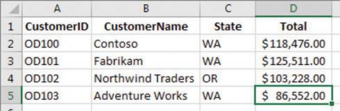
A list of data that contains customer information
If you want to find the average order of customers from the state of Washington (abbreviated in the worksheet as WA), you can create the formula =AVERAGEIF(C3:C6, “WA”, D3:D6).
The AVERAGEIFS, SUMIFS, and COUNTIFS functions extend the capabilities of the AVERAGEIF, SUMIF, and COUNTIF functions to allow for multiple criteria. If you want to find the sum of all orders of at least $100,000 placed by companies in Washington, you can create the formula=SUMIFS(D3:D6, C3:C6, “=WA”, D3:D6, “>=100000”).
The AVERAGEIFS and SUMIFS functions start with a data range that contains values that the formula summarizes; you then list the data ranges and the criteria to apply to that range. In generic terms, the syntax runs =AVERAGEIFS(data_range, criteria_range1, criteria1[,criteria_range2, criteria2...]). The part of the syntax in brackets (which aren’t used when you create the formula) is optional, so an AVERAGEIFS or SUMIFS formula that contains a single criterion will work. The COUNTIFS function, which doesn’t perform any calculations, doesn’t need a data range—you just provide the criteria ranges and criteria. For example, you could find the number of customers from Washington who were billed at least $100,000 by using the formula =COUNTIFS(D3:D6, “=WA”, E3:E6, “>=100000”).
To summarize data by using the IF function
1. Click the cell in which you want to enter the formula.
2. Enter a formula with the syntax =IF(Logical_test, Value_if_true, Value_if_false) where:
• Logical_test is the logical test to be performed.
• Value_if_true is the value the formula returns if the test is true.
• Value_if_false is the value the formula returns if the test is false.
To create a formula by using the Insert Function dialog box
1. To the left of the formula bar, click the Insert Function button.
2. In the Insert Function dialog box, click the function you want to use in your formula.
3. Click OK.
4. In the Function Arguments dialog box, define the arguments for the function you chose.
5. Click OK.
To count cells that contain numbers in a range
1. Click the cell in which you want to enter the formula.
2. Create a formula with the syntax =COUNT(range), where range is the cell range in which you want to count cells.
To count cells that are non-blank
1. Click the cell in which you want to enter the formula.
2. Create a formula with the syntax =COUNTA(range), where range is the cell range in which you want to count cells.
To count cells that contain a blank value
1. Click the cell in which you want to enter the formula.
2. Create a formula with the syntax =COUNTBLANK(range), where range is the cell range in which you want to count cells.
To count cells that meet one condition
1. Click the cell in which you want to enter the formula.
2. Enter a formula of the form =COUNTIF(range, criteria) where:
• range is the cell range that might contain the criteria value.
• criteria is the logical test used to determine whether to count the cell or not.
To count cells that meet multiple conditions
1. Click the cell in which you want to enter the formula.
2. Enter a formula of the form =COUNTIFS(criteria_range, criteria,...) where for each criteria_range and criteria pair:
• criteria_range is the cell range that might contain the criteria value.
• criteria is the logical test used to determine whether to count the cell or not.
To find the sum of data that meets one condition
1. Click the cell in which you want to enter the formula.
2. Enter a formula of the form =SUMIF(range, criteria, sum_range) where:
• range is the cell range that might contain the criteria value.
• criteria is the logical test used to determine whether to include the cell or not.
• sum_range is the range that contains the values to be included if the range cell in the same row meets the criterion.
To find the sum of data that meets multiple conditions
1. Click the cell in which you want to enter the formula.
2. Enter a formula of the form =SUMIFS(sum_range, criteria_range, criteria,...) where:
• sum_range is the range that contains the values to be included if all criteria_range cells in the same row meet all criteria.
• criteria_range is the cell range that might contain the criteria value.
• criteria is the logical test used to determine whether to include the cell or not.
To find the average of data that meets one condition
1. Click the cell in which you want to enter the formula.
2. Enter a formula of the form =AVERAGEIF(range, criteria, average_range) where:
• range is the cell range that might contain the criteria value.
• criteria is the logical test used to determine whether to include the cell or not.
• average_range is the range that contains the values to be included if the range cell in the same row meets the criterion.
To find the average of data that meets multiple conditions
1. Click the cell in which you want to enter the formula.
2. Enter a formula of the form =AVERAGEIFS(average_range, criteria_range, criteria,...) where:
• average_range is the range that contains the values to be included if all criteria_range cells in the same row meet all criteria.
• criteria_range is the cell range that might contain the criteria value.
• criteria is the logical test used to determine whether to include the cell or not.
To display a custom message if a cell contains an error
1. Click the cell in which you want to enter the formula.
2. Enter a formula with the syntax =IFERROR(value, value_if_error) where:
• value is a cell reference or formula.
• value_if_error is the value to be displayed if the value argument returns an error.
Set iterative calculation options and enable or disable automatic calculation
Excel formulas use values in other cells to calculate their results. If you create a formula that refers to the cell that contains the formula, you have created a circular reference. Under most circumstances, Excel treats circular references as a mistake for two reasons. First, the vast majority of Excel formulas don’t refer to their own cell, so a circular reference is unusual enough to be identified as an error. The second, more serious consideration is that a formula with a circular reference can slow down your workbook. Because Excel repeats, or iterates, the calculation, you need to set limits on how many times the app repeats the operation.
You can control your workbook’s calculation options by using the controls on the Formulas page of the Excel Options dialog box.
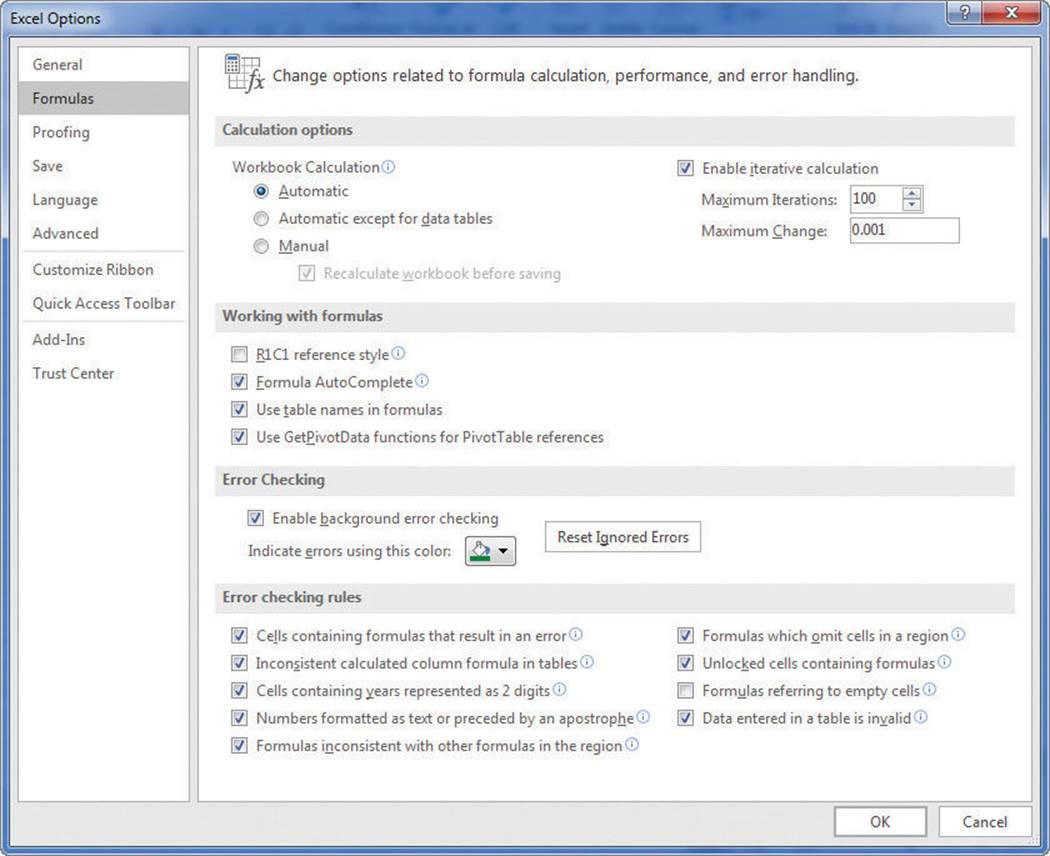
Set iterative calculation options on the Formulas page of the Excel Options dialog box
The Calculation Options section of the Excel Options dialog box has three available settings:
![]() Automatic The default setting; recalculates a worksheet whenever a value affecting a formula changes
Automatic The default setting; recalculates a worksheet whenever a value affecting a formula changes
![]() Automatic except for data tables Recalculates a worksheet whenever a value changes, but doesn’t recalculate data tables
Automatic except for data tables Recalculates a worksheet whenever a value changes, but doesn’t recalculate data tables
![]() Manual Requires you to press F9 or, on the Formulas tab, in the Calculation group, click the Calculate Now button to recalculate your worksheet
Manual Requires you to press F9 or, on the Formulas tab, in the Calculation group, click the Calculate Now button to recalculate your worksheet
You can also use options in the Calculation Options section to allow or disallow iterative calculations. If you select the Enable Iterative Calculation check box, Excel repeats calculations for cells that contain formulas with circular references. The default Maximum Iterations value of 100 and Maximum Change of 0.001 are appropriate for all but the most unusual circumstances.
![]() Tip
Tip
You can also control when Excel recalculates its formulas by clicking the Formulas tab on the ribbon, clicking the Calculation Options button, and selecting the behavior you want.
To recalculate a workbook
1. Display the workbook you want to recalculate.
2. Press F9.
Or
On the Formulas tab, in the Calculation group, click Calculate Now.
To recalculate a worksheet
1. Display the worksheet you want to recalculate.
2. In the Calculation group, click the Calculate Sheet button.
To set worksheet calculation options
1. Display the worksheet whose calculation options you want to set.
2. In the Calculation group, click the Calculate Options button.
3. Click the calculation option you want in the list.
To set iterative calculation options
1. Display the Backstage view, and then click Options.
2. In the Excel Options dialog box, click Formulas.
3. In the Calculation options section, select or clear the Enable iterative calculation check box.
4. In the Maximum Iterations box, enter the maximum iterations allowed for a calculation.
5. In the Maximum Change box, enter the maximum change allowed for each iteration.
6. Click OK.
Use array formulas
Most Excel formulas calculate values to be displayed in a single cell. For example, you could add the formulas =B1*B4, =B1*B5, and =B1*B6 to consecutive worksheet cells to calculate shipping insurance costs based on the value of a package’s contents.
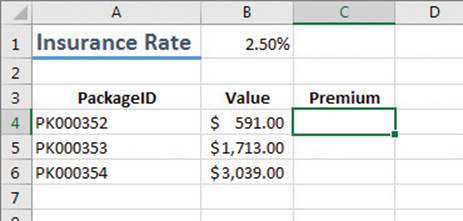
A worksheet with data to be summarized by an array formula
Rather than add the same formula to multiple cells one cell at a time, you can add a formula to every cell in the target range at the same time by creating an array formula. To create an array formula, you enter the formula’s arguments and press Ctrl+Shift+Enter to identify the formula as an array formula. To calculate package insurance rates for values in the cell range B4:B6 and the rate in cell B1, you would select a range of cells with the same shape as the value range and enter the formula =B1*B4:B6. In this case, the values are in a three-cell column, so you must select a range of the same shape, such as C4:C6.
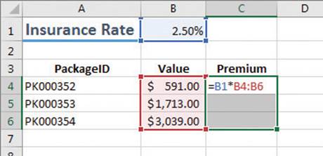
A worksheet with an array formula ready to be entered
![]() Important
Important
If you enter the array formula into a range of the wrong shape, Excel displays duplicate results, incomplete results, or error messages, depending on how the target range differs from the value range.
When you press Ctrl+Shift+Enter, Excel creates an array formula in the selected cells. The formula appears within a pair of braces to indicate that it is an array formula.
![]() Important
Important
You can’t add braces to a formula to make it an array formula—you must press Ctrl+Shift+Enter to create it.
In addition to creating an array formula that combines a single cell’s value with an array, you can create array formulas that use two separate arrays. For example, a company might establish a goal to reduce sorting time in each of four distribution centers.
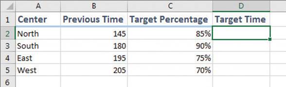
A worksheet with data for an array formula that multiplies two arrays
This worksheet stores the previous sorting times in minutes in cells B2:B5, and the percentage targets in cells C2:C5. The array formula to calculate the targets for each of the four centers is =B2:B5*C2:C5 which, when entered into cells D2:D5 by pressing Ctrl+Shift+Enter, would appear as{= B2:B5*C2:C5}.
To edit an array formula, you must select every cell that contains the array formula, click the formula bar to activate it, edit the formula in the formula bar, and then press Ctrl+Shift+Enter to re-enter the formula as an array formula.
![]() Tip
Tip
Many operations that used to require an array formula can now be calculated by using functions such as SUMIFS and COUNTIFS.
To create an array formula
1. Select the cells into which you want to enter the array formula.
2. Enter your array formula.
3. Press Ctrl+Shift+Enter.
To edit an array formula
1. Select the cells that contain the array formula.
2. Edit your array formula.
3. Press Ctrl+Shift+Enter.
Find and correct errors in calculations
Including calculations in a worksheet gives you valuable answers to questions about your data. As is always true, however, it is possible for errors to creep into your formulas. With Excel, you can find the source of errors in your formulas by identifying the cells used in a specific calculation and describing any errors that have occurred. The process of examining a worksheet for errors is referred to as auditing.
Excel identifies errors in several ways. The first way is to display an error code in the cell holding the formula generating the error.
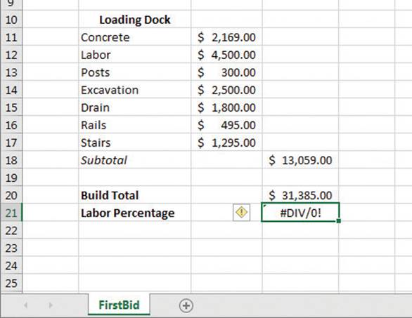
A worksheet with an error code displayed
When a cell with an erroneous formula is the active cell, an Error button is displayed next to it. If you point to the Error button Excel displays an arrow on the button’s right edge. Clicking the arrow displays a menu with options that provide information about the error and offer to help you fix it.
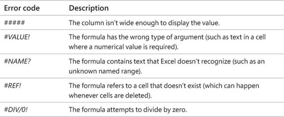
The following table lists the most common error codes and what they mean.
Another technique you can use to find the source of formula errors is to ensure that the appropriate cells are providing values for the formula. You can identify the source of an error by having Excel trace a cell’s precedents, which are the cells with values used in the active cell’s formula. You can also audit your worksheet by identifying cells with formulas that use a value from a particular cell. Cells that use another cell’s value in their calculations are known as dependents, meaning that they depend on the value in the other cell to derive their own value.
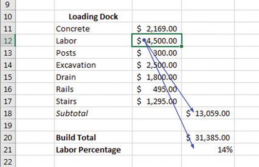
A worksheet with a cell’s dependents indicated by tracer arrows
If the cells identified by the tracer arrows aren’t the correct cells, you can hide the arrows and correct the formula.
If you prefer to have the elements of a formula error presented as text in a dialog box, you can use the Error Checking dialog box to move through the formula one step at a time, to choose to ignore the error, or to move to the next or the previous error.
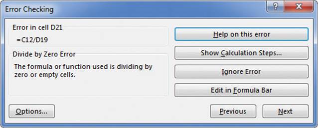
Identify and manage errors by using the Error Checking dialog box
![]() Tip
Tip
You can have the Error Checking tool ignore formulas that don’t use every cell in a region (such as a row or column) by modifying this option in the Excel Options dialog box. To do so, on the Formulas tab of the dialog box, if you clear the Formulas Which Omit Cells In A Region check box, you can create formulas that don’t add up every value in a row or column (or rectangle) without Excel marking them as an error.
For times when you just want to display the results of each step of a formula and don’t need the full power of the Error Checking tool, you can use the Evaluate Formula dialog box to move through each element of the formula. The Evaluate Formula dialog box is much more useful for examining formulas that don’t produce an error but aren’t generating the result you expect.
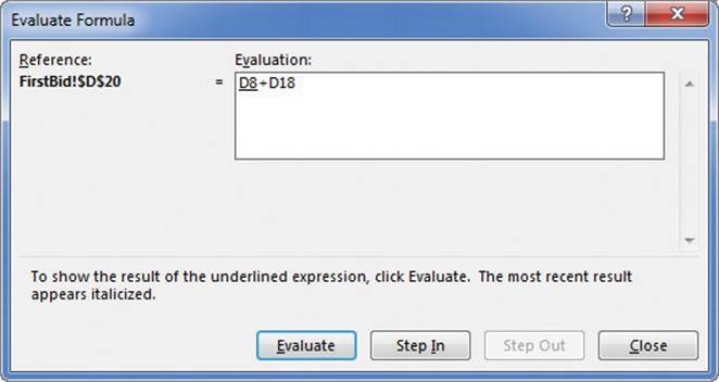
Step through formulas by using the Evaluate Formula dialog box
Finally, you can monitor the value in a cell regardless of where in your workbook you are by opening a Watch Window that displays the value in the cell. For example, if one of your formulas uses values from cells in other worksheets or even other workbooks, you can set a watch on the cell that contains the formula and then change the values in the other cells.
As soon as you enter the new value, the Watch Window displays the new result of the formula. When you’re done watching the formula, you can delete the watch and hide the Watch Window.
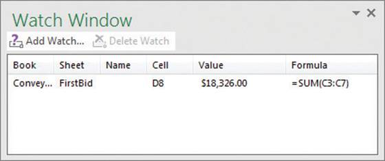
Follow cell values by using the Watch Window
To display information about a formula error
1. Click the cell that contains the error.
2. Point to the error indicator next to the cell.
Or
Click the error indicator to display more information.
To display arrows identifying formula precedents
1. On the Formulas tab, in the Formula Auditing group, click the Trace Precedents button.
To display arrows identifying cell dependents
1. In the Formula Auditing group, click the Trace Dependents button.
To remove tracer arrows
1. Do either of the following:
• In the Formula Auditing group, click the Remove Arrows button (not its arrow).
• Click the Remove Arrows arrow and select the arrows you want to remove.
To move through a calculation one step at a time
1. Click the cell that contains the formula you want to evaluate.
2. In the Formula Auditing group, click the Evaluate Formula button.
3. In the Evaluate Formula dialog box, click Evaluate.
4. Click Step In to move forward by one calculation.
Or
Click Step Out to move backward by one calculation.
5. Click Close.
To change error display options
1. Display the Backstage view, and then click Options.
2. In the Excel Options dialog box, click Formulas.
3. In the Error Checking section, select or clear the Enable background error checking check box.
4. Click the Indicate errors using this color button and select a color.
5. Click Reset Ignored Errors to return Excel to its default error indicators.
6. In the Error checking rules section, select or clear the check boxes next to errors you want to indicate or ignore, respectively.
To watch the values in a cell range
1. Click the cell range you want to watch.
2. In the Formula Auditing group, click the Watch Window button.
3. In the Watch Window dialog box, click Add Watch.
4. Click Add.
To delete a watch
1. Click the Watch Window button.
2. In the Watch Window dialog box, click the watch you want to delete.
3. Click Delete Watch.
Skills review
In this chapter, you learned how to:
![]() Name groups of data
Name groups of data
![]() Create formulas to calculate values
Create formulas to calculate values
![]() Summarize data that meets specific conditions
Summarize data that meets specific conditions
![]() Set iterative calculation options and enable or disable automatic calculation
Set iterative calculation options and enable or disable automatic calculation
![]() Use array formulas
Use array formulas
![]() Find and correct errors in calculations
Find and correct errors in calculations
 Practice tasks
The practice files for these tasks are located in the Excel2016SBS\Ch03 folder. You can save the results of the tasks in the same folder.
Name groups of data
Open the CreateNames workbook in Excel, and then perform the following tasks:
1. Create a named range named Monday for the V_101 through V_109 values (found in cells C4:C12) for that weekday.
2. Edit the Monday named range to include the V_110 value for that column.
3. Select cells B4:H13 and create named ranges for V_101 through V_110, drawing the names from the row headings.
4. Delete the Monday named range.
Create formulas to calculate values
Open the BuildFormulas workbook in Excel, and then perform the following tasks:
1. On the Summary worksheet, in cell F9, create a formula that displays the value from cell C4.
2. Edit the formula in cell F9 so it uses the SUM function to find the total of values in cells C3:C8.
3. In cell F10, create a formula that finds the total expenses for desktop software and server software.
4. Edit the formula in F10 so the cell references are absolute references.
5. On the JuneLabor worksheet, in cell F13, create a SUM formula that finds the total of values in the JuneSummary table’s Labor Expense column.
Summarize data that meets specific conditions
Open the CreateConditionalFormulas workbook in Excel, and then perform the following tasks:
1. In cell G3, create an IF formula that tests whether the value in F3 is greater than or equal to 35,000. If it is, display Request discount; if not, display No discount available.
2. Copy the formula from cell G3 to the range G4:G14.
3. In cell I3, create a formula that finds the average cost of all expenses in cells F3:F14 where the Type column contains the value Box.
4. In cell I6, create a formula that finds the sum of all expenses in cells F3:F14 where the Type column contains the value Envelope and the Destination column contains the value International.
Set iterative calculation options and enable or disable automatic calculation
Open the SetIterativeOptions workbook in Excel, and then perform the following tasks:
1. On the Formulas tab, in the Calculation group, click the Calculation Options button, and then click Manual.
2. In cell B6, enter the formula =B7*B9, and then press Enter.
Note that this result is incorrect because the Gross Savings minus the Savings Incentive should equal the Net Savings value, which it does not.
3. Press F9 to recalculate the workbook and read the message box indicating you have created a circular reference.
4. Click OK.
5. Use options in the Excel Options dialog box to enable iterative calculation.
6. Close the Excel Options dialog box and recalculate the worksheet.
7. Change the workbook’s calculation options to Automatic.
Use array formulas
Open the CreateArrayFormulas workbook in Excel, and then perform the following tasks:
1. On the Fuel worksheet, select cells C11:F11.
2. Enter the array formula =C3*C9:F9 in the selected cells.
3. Edit the array formula you just created to read =C3*C10:F10.
4. Display the Volume worksheet.
5. Select cells D4:D7.
6. Create the array formula =B4:B7*C4:C7.
Find and correct errors in calculations
Open the AuditFormulas workbook in Excel, and then perform the following tasks:
1. Create a watch that displays the value in cell D20.
2. Click cell D8, and then display the formula’s precedents.
3. Remove the tracer arrows from the worksheet.
4. Click cell A1, and then use the Error Checking dialog box to identify the error in cell D21.
5. Show the tracer arrows for the error.
6. Remove the arrows, then edit the formula in cell D21 so it is =C12/D20.
7. Use the Evaluate Formula dialog box to evaluate the formula in cell D21.
8. Delete the watch you created in step 1.
All materials on the site are licensed Creative Commons Attribution-Sharealike 3.0 Unported CC BY-SA 3.0 & GNU Free Documentation License (GFDL)
If you are the copyright holder of any material contained on our site and intend to remove it, please contact our site administrator for approval.
© 2016-2026 All site design rights belong to S.Y.A.