Microsoft Excel 2016 Step by Step (2015)
Part 2: Analyze and present data
CHAPTER 5
Manage worksheet data
CHAPTER 6
Reorder and summarize data
CHAPTER 7
Combine data from multiple sources
CHAPTER 8
Analyze alternative data sets
CHAPTER 9
Create charts and graphics
CHAPTER 10
Create dynamic worksheets by using PivotTables
5. Manage worksheet data
In this chapter
![]() Limit data that appears on your screen
Limit data that appears on your screen
![]() Manipulate worksheet data
Manipulate worksheet data
![]() Define valid sets of values for ranges of cells
Define valid sets of values for ranges of cells
Practice files
For this chapter, use the practice files from the Excel2016SBS\Ch05 folder. For practice file download instructions, see the introduction.
With Excel 2016, you can manage huge data collections, but storing more than 1 million rows of data doesn’t help you make business decisions unless you have the ability to focus on the most important data in a worksheet. Focusing on the most relevant data in a worksheet facilitates decision making. Excel includes many powerful and flexible tools with which you can limit the data displayed in your worksheet. When your worksheet displays the subset of data you need to make a decision, you can perform calculations on that data. You can discover what percentage of monthly revenue was earned in the 10 best days in the month, find your total revenue for particular days of the week, or locate the slowest business day of the month.
Just as you can limit the data displayed by your worksheets, you can also create validation rules that limit the data entered into them. When you set rules for data entered into cells, you can catch many of the most common data entry errors, such as entering values that are too small or too large, or attempting to enter a word in a cell that requires a number. If you add a validation rule after data has been entered, you can circle any invalid data so that you know what to correct.
This chapter guides you through procedures related to limiting the data that appears on your screen, manipulating list data, and creating validation rules that limit data entry to appropriate values.
Limit data that appears on your screen
Excel worksheets can hold as much data as you need them to, but you might not want to work with all the data in a worksheet at the same time. For example, you might want to look at the revenue figures for your company during the first third, second third, and final third of a month. You can limit the data shown on a worksheet by creating a filter, which is a rule that selects rows to be shown in a worksheet.
![]() Important
Important
When you turn on filtering, Excel treats the cells in the active cell’s column as a range. To ensure that the filtering works properly, you should always have a label at the top of the column you want to filter. If you don’t, Excel treats the first value in the list as the label and doesn’t include it in the list of values by which you can filter the data.
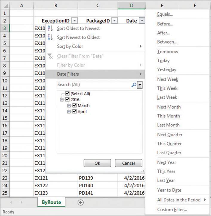
When you turn on filtering, a filter arrow appears to the right of each column label in the list of data. Clicking the filter arrow displays a menu of filtering options and a list of the unique values in the column. Each item has a check box next to it, which you can use to create a selection filter. Some of the commands vary depending on the type of data in the column. For example, if the column contains a set of dates, you will get a list of commands specific to that data type.
![]() Tip
Tip
In Excel tables, filter arrows are turned on by default.
![]() Tip
Tip
When a column contains several types of data, the filter command for it is Number Filters.
Use filters to limit the data that appears in a worksheet
When you click a filtering option, Excel displays a dialog box in which you can define the filter’s criteria. As an example, you could create a filter that displays only dates after 3/31/2016.
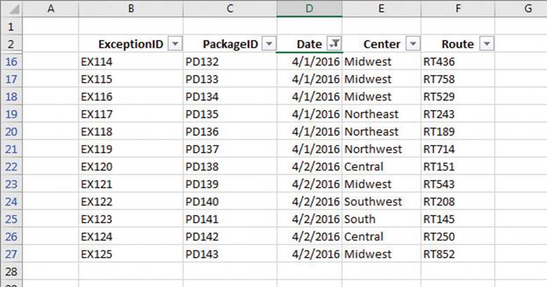
Columns with a filter applied display a funnel icon on their filter arrows
If you want to display the highest or lowest values in a data column, you can create a Top 10 filter. You can choose whether to show values from the top or bottom of the list, define the number of items you want to display, and choose whether that number indicates the actual number of items or the percentage of items to be shown when the filter is applied.
![]() Tip
Tip
Top 10 filters can be applied only to columns that contain number values.
Excel 2016 includes a capability called the search filter, which you can use to enter a search string that Excel uses to identify which items to display in an Excel table or a data list. Enter the character string you want to search for, and Excel limits your data to values that contain that string.
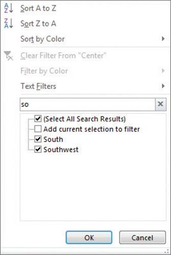
Applying a search filter limits the items that appear in the selection list
When you create a custom filter, you can define a rule that Excel uses to decide which rows to show after the filter is applied. For instance, you can create a rule that determines that only days with package volumes of less than 100,000 should be shown in your worksheet. With those results in front of you, you might be able to determine whether the weather or another factor resulted in slower business on those days.
Excel indicates that a column has a filter applied by changing the appearance of the column’s filter arrow to include an icon that looks like a funnel. After you finish examining your data by using a filter, you can clear the filter or turn off filtering entirely and hide the filter arrows.
To turn on filter arrows
1. Click any cell in the list of data you want to filter.
2. On the Home tab of the ribbon, in the Editing group, click Sort & Filter, and then click Filter.
To create a selection filter
1. Click Sort & Filter, and then click Filter.
2. Click the filter arrow for the column by which you want to filter your data.
3. Clear the check boxes next to the items you want to hide.
Or
Clear the Select All check box and select the check boxes next to the items you want to display.
4. Click OK.
To create a filter rule
1. Display the filter arrows for your list of data.
2. Click the filter arrow for the field by which you want to filter your data.
3. Point to the Type Filters item to display the available filters for the column’s data type.
4. Click the filter you want to create.
5. Enter the arguments required to define the rule.
6. Click OK.
To create a Top 10 filter
1. Display the filter arrows for your list of data.
2. Click the filter arrow for a column that contains number values, point to Number Filters, and then click Top 10.
3. In the Top 10 AutoFilter dialog box, click the arrow for the first list box, and select whether to display the top or bottom values.
4. Click the arrow for the last list box, and select whether to base the rule on the number of items or the percentage of items.
5. Click in the middle box and enter the number or percentage of items to display.
6. Click OK.
To create a search filter
1. Display the filter arrows for your list of data.
2. Click the filter arrow for the field by which you want to filter your data.
3. Enter the character string that should appear in the values you want to display in the filter list.
4. Click OK.
To clear a filter
1. Click the filter arrow for the field that has the filter you want to clear.
2. Click Clear Filter From Field.
To turn off the filter arrows
1. Click any cell in the list of data.
2. Click Sort & Filter, and then click Filter.
Manipulate worksheet data
Excel includes a wide range of tools you can use to summarize worksheet data. This topic describes how to select rows at random by using the RAND and RANDBETWEEN functions, how to summarize worksheet data by using the SUBTOTAL and AGGREGATE functions, and how to display a list of unique values within a data set.
Select list rows at random
In addition to filtering the data that is stored in your Excel worksheets, you can choose rows at random from a list. Selecting rows randomly is useful for choosing which customers will receive a special offer, deciding which days of the month to audit, or picking prize winners at an employee party.
To choose rows randomly, you can use the RAND function, which generates a random decimal value between 0 and 1, and compare the value it returns with a test value included in a formula. If you recalculate the RAND function 10 times and check each time to find out whether the value is below 0.3, it’s very unlikely that you would get exactly three instances where the value is below 0.3. Just as flipping a coin can result in the same result 10 times in a row by chance, so can the RAND function’s results appear to be off if you only recalculate it a few times. However, if you were to recalculate the function 10,000 times, it is extremely likely that the number of values less than 0.3 would be very close to 30 percent.
TIP Because the RAND function is a volatile function (that is, it recalculates its results every time you update the worksheet), you should copy the cells that contain the RAND function in a formula and paste the formulas’ values back into their original cells. To do so, select the cells that contain the RAND formulas and paste them back into the same cells as values.
The RANDBETWEEN function generates a random whole number within a defined range. For example, the formula =RANDBETWEEN(1,100) would generate a random integer value from 1 through 100, inclusive. The RANDBETWEEN function is very useful for creating sample data collections for presentations. Before the RANDBETWEEN function was introduced, you had to create formulas that added, subtracted, multiplied, and divided the results of the RAND function, which are always decimal values between 0 and 1, to create data.
To use RAND or RANDBETWEEN to select a row, create an IF formula that tests the random values. If you want to check 30 percent of the rows, a formula such as =IF(cell_address<0.3, “TRUE”, “FALSE”) would display TRUE in the formula cells for any value of 0.3 or less and FALSE otherwise.
Summarize data in worksheets that have hidden and filtered rows
The ability to analyze the data that’s most vital to your current needs is important, but there are some limitations to how you can summarize your filtered data by using functions such as SUM and AVERAGE. One limitation is that any formulas you create that include the SUM and AVERAGEfunctions don’t change their calculations if some of the rows used in the formula are hidden by the filter.
Excel provides two ways to summarize just the visible cells in a filtered data list. The first method is to use AutoCalculate. To use AutoCalculate, you select the cells you want to summarize. When you do, Excel displays the average of the values in the cells, the sum of the values in the cells, and the number of visible cells (the count) in the selection. You’ll find the display on the status bar at the lower edge of the Excel window.
When you use AutoCalculate, you aren’t limited to finding the sum, average, and count of the selected cells. You can add or remove calculations to suit your needs; a check mark appears next to a function’s name if that function’s result appears on the status bar.
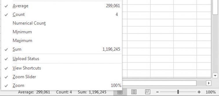
The status bar displays summary values when you select more than one cell that contains numeric data
AutoCalculate is great for finding a quick total or average for filtered cells, but it doesn’t make the result available in the worksheet. Formulas such as =SUM(C3:C26) always consider every cell in the range, regardless of whether you hide a cell’s row manually or not, so you need to create a formula by using either the SUBTOTAL function or the AGGREGATE function to summarize just those values that are visible in your worksheet. The SUBTOTAL function lets you choose whether to summarize every value in a range or summarize only those values in rows you haven’t manually hidden. The SUBTOTAL function has this syntax: =SUBTOTAL(function_num, ref1, ref2, ...). The function_num argument holds the number of the operation you want to use to summarize your data. (The operation numbers are summarized in a table later in this section.) The ref1,ref2, and further arguments represent up to 29 ranges to include in the calculation.
As an example, assume you have a worksheet where you hid rows 20-26 manually. In this case, the formula =SUBTOTAL(9, C3:C26, E3:E26, G3:G26) would find the sum of all values in the ranges C3:C26, E3:E26, and G3:G26, regardless of whether that range contained any hidden rows. The formula =SUBTOTAL(109, C3:C26, E3:E26, G3:G26) would find the sum of all values in cells C3:C19, E3:E19, and G3:G19, ignoring the values in the manually hidden rows.
![]() Important
Important
Be sure to place your SUBTOTAL formula in a row that is even with or above the headers in the range you’re filtering. If you don’t, your filter might hide the formula’s result!
The following table lists the summary operations available for the SUBTOTAL formula. Excel displays the available summary operations as part of the Formula AutoComplete functionality, so you don’t need to remember the operation numbers or look them up in the Help system.
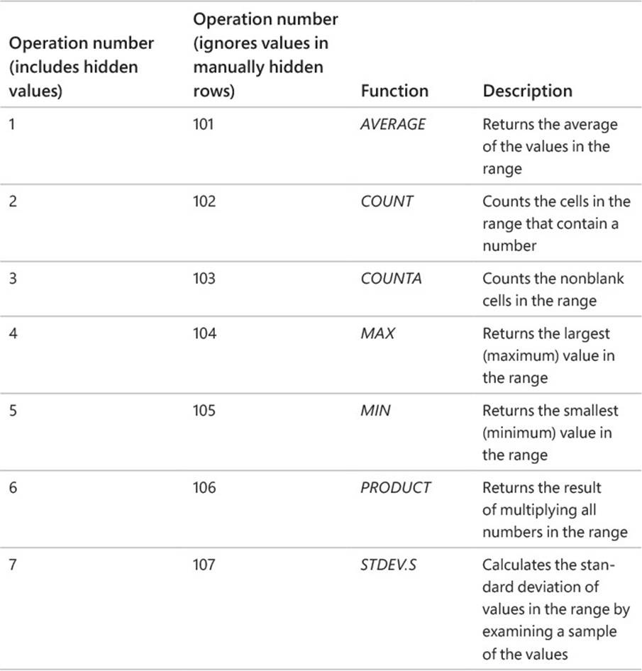
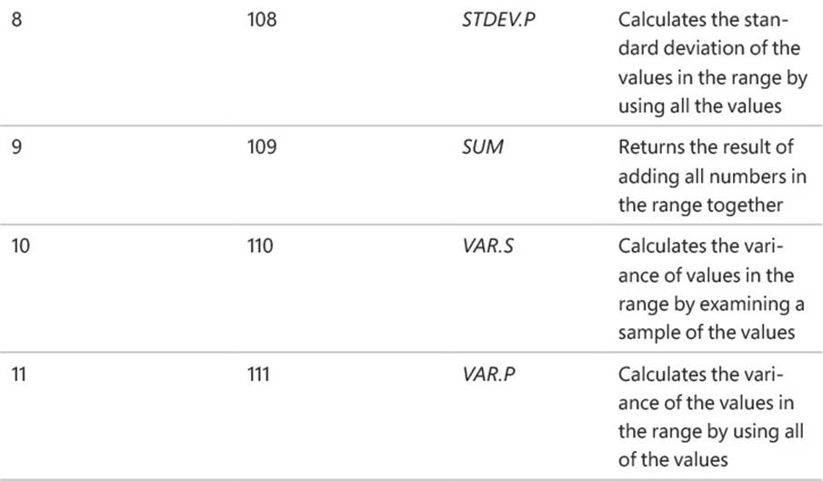
As the preceding table shows, the SUBTOTAL function has two sets of operations. The first set (operations 1-11) represents operations that include hidden values in their summary, and the second set (operations 101-111) represents operations that summarize only values visible in the worksheet. Operations 1-11 summarize all cells in a range, regardless of whether the range contains any manually hidden rows. By contrast, operations 101-111 ignore any values in manually hidden rows. What the SUBTOTAL function doesn’t do, however, is change its result to reflect rows hidden by using a filter.
![]() Important
Important
Excel treats the first cell in the data range as a header cell, so it doesn’t consider the cell as it builds the list of unique values. Be sure to include the header cell in your data range!
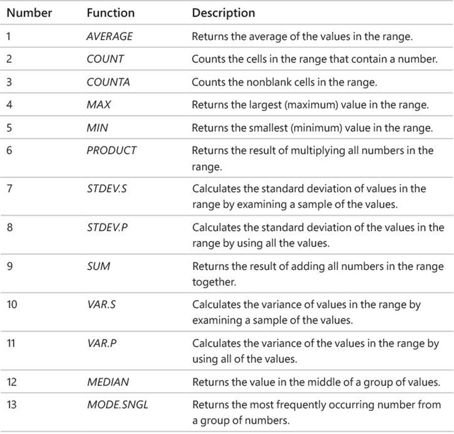
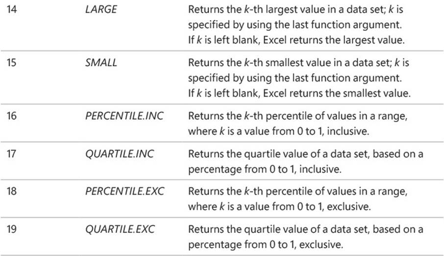
The AGGREGATE function extends the capabilities of the SUBTOTAL function. With it, you can select from a broader range of functions and use another argument to determine which, if any, values to ignore in the calculation. AGGREGATE has two possible syntaxes, depending on the summary operation you select. The first syntax is =AGGREGATE(function_num, options, ref1...), which is similar to the syntax of the SUBTOTAL function. The other possible syntax, =AGGREGATE(function_num, options, array, [k]), is used to create AGGREGATE functions that use theLARGE, SMALL, PERCENTILE.INC, QUARTILE.INC, PERCENTILE.EXC, and QUARTILE.EXC operations.
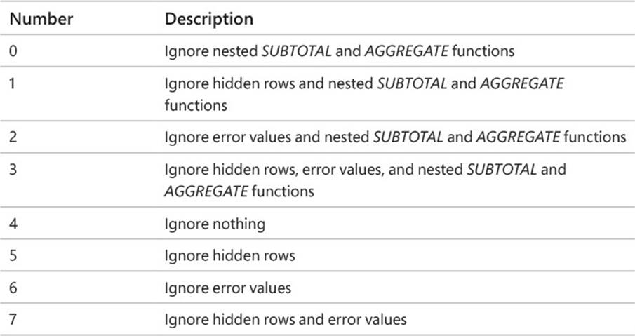
The following table summarizes the summary operations available for use in the AGGREGATE function.
You use the second argument, options, to select which items the AGGREGATE function should ignore. These items can include hidden rows, errors, and SUBTOTAL and AGGREGATE functions. The following table summarizes the values available for the options argument and the effect they have on the function’s results.
To summarize values by using AutoCalculate
1. Select the cells in your worksheet.
2. View the summaries on the status bar.
To change the AutoCalculate summaries displayed on the status bar
1. Right-click the status bar.
2. Click a summary operation without a check mark to display it.
Or
Click a summary operation with a check mark to hide it.
To create a SUBTOTAL formula
1. In a cell, enter a formula that uses the syntax =SUBTOTAL(function_num, ref1, ref2, ...). The arguments in the syntax are as follows:
• The function_num argument is the reference number of the function you want to use.
• The ref1, ref2, and subsequent ref arguments refer to cell ranges.
To create an AGGREGATE formula
1. Do one of the following:
• Create a formula of the syntax =AGGREGATE(function_num, options, ref1...). The arguments in the syntax are as follows:
• The function_num argument is the reference number of the function you want to use.
• The options argument is the reference number for the options you want.
• The ref1, ref2, and subsequent ref arguments refer to cell ranges.
Or
• Create a formula with the syntax =AGGREGATE(function_num, options, array, [k]). The arguments in the syntax are as follows:
• The function_num argument is the reference number of the function you want to use.
• The options argument is the reference number for the options you want to use.
• The array argument represents the cell range (array) that provides data for the formula.
• The optional k argument, used with the LARGE, SMALL, PERCENTILE.INC, QUARTILE.INC, PERCENTILE.EXC, and QUARTILE.EXC, indicates which value, percentile, or quartile to return.
Find unique values within a data set
Summarizing numerical values can provide valuable information that helps you run your business. It can also be helpful to know how many different values appear within a column. For example, you might want to display all of the countries and regions in which Consolidated Messenger has customers. If you want to display a list of the unique values in a column, you can do so by creating an advanced filter.
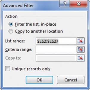
Use the Advanced Filter dialog box to find unique records in a list
All you need to do is identify the rows that contain the values you want to filter and indicate that you want to display unique records so that you get only the information you want.
To find unique values within a data set
1. Click any cell in the range for which you want to find unique values.
2. On the Data tab of the ribbon, in the Sort & Filter group, click Advanced.
3. Click Filter the list, in place.
Or
Click Copy to another location.
4. Verify that the address of your data range appears in the List range box.
5. If necessary, click in the Copy to box and select the cells where you want the filtered list to appear.
6. Select the Unique records only check box.
7. Click OK.
Define valid sets of values for ranges of cells
Part of creating efficient and easy-to-use worksheets is to do what you can to ensure that the data entered into your worksheets is as accurate as possible. Although it isn’t possible to catch every typographical or transcription error, you can set up a validation rule to make sure that the data entered into a cell meets certain standards. For example, you can specify the type of data you want, the range of acceptable values, and whether blank values are allowed. Setting accurate validation rules can help you and your colleagues avoid entering a customer’s name in the cell designated to hold the phone number or setting a credit limit above a certain level.
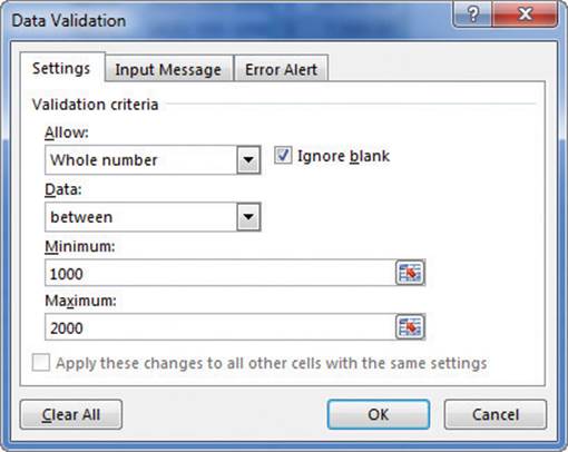
Create data validation rules to ensure that appropriate data is entered into worksheet cells
You can select the cells where you want to add a validation rule, even if those cells already contain data. Excel doesn’t tell you whether any of those cells contain data that violates your rule at the moment you create the rule, but you can find out by having Excel circle any worksheet cells that contain data that violates the cell’s validation rule. When you’re done, you can have Excel clear the validation circles or have Excel turn off data validation for those cells entirely.
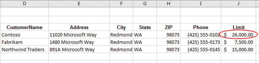
Validation circles indicate data previously entered into a worksheet that violates data validation rules
To add a validation rule to a cell
1. On the Data tab, in the Data Tools group, click Data Validation.
2. In the Data Validation dialog box, on the Settings tab, click the Allow arrow, and then click the type of values to allow.
3. Use the controls to define the rule.
4. Select the Ignore blank check box to allow blank values.
Or
Clear the Ignore blank check box to require a value be entered.
5. On the Input Message tab, enter an input message for the cell.
6. On the Error Alert tab, create an error alert message for values that violate the rule.
7. Click OK.
To edit a validation rule
1. Select one or more cells that contain the validation rule.
2. Click Data Validation.
3. On the Settings tab, select the Apply these changes to all other cells with the same settings check box to affect other cells with the same rule.
Or
Leave the Apply these changes to all other cells with the same settings check box cleared to affect only the selected cells.
4. Use the controls in the dialog box to edit the rule, input message, and error alert.
5. Click OK.
To circle invalid data in a worksheet
1. Click the Data Validation arrow.
2. Click Circle Invalid Data.
To remove validation circles
1. Click the Data Validation arrow.
2. Click Clear Validation Circles.
Skills review
In this chapter, you learned how to:
![]() Limit data that appears on your screen
Limit data that appears on your screen
![]() Manipulate worksheet data
Manipulate worksheet data
![]() Define valid sets of values for ranges of cells
Define valid sets of values for ranges of cells
 Practice tasks
The practice files for these tasks are located in the Excel2016SBS\Ch05 folder. You can save the results of the tasks in the same folder.
Limit data that appears on your screen
Open the LimitData workbook in Excel, and then perform the following tasks:
1. Create a filter that displays only those package exceptions that happened on RT189.
2. Clear the previous filter, and then create a filter that shows exceptions for the Northeast and Northwest centers.
3. With the previous filter still in place, create a filter that displays only those exceptions that occurred before April 1, 2016.
4. Clear the filter that shows values related to the Northeast and Northwest centers.
5. Turn off filtering for the list of data.
Manipulate worksheet data
Open the SummarizeValues workbook in Excel, and then perform the following tasks:
1. Combine the IF and RAND functions into formulas in cells H3:H27 that display TRUE if the value is less than 0.3 and FALSE otherwise.
2. Use AutoCalculate to find the SUM, AVERAGE, and COUNT of cells G12:G16.
3. Remove the COUNT summary from the status bar and add the MINIMUM summary.
4. Create a SUBTOTAL formula that finds the average of the values in cells G3:G27.
5. Create an AGGREGATE formula that finds the maximum of values in cells G3:G27.
6. Create an advanced filter that finds the unique values in cells F3:F27.
Define valid sets of values for ranges of cells
Open the ValidateData workbook in Excel, and then perform the following tasks:
1. Create a data validation rule in cells J4:J7 that requires values entered into those cells be no greater than $25,000.
2. Attempt to type the value 30000 in cell J7, observe the message that appears, and then cancel data entry.
3. Edit the rule you created so it includes an input message and an error alert.
4. Display validation circles to highlight data that violates the rule you created, and then hide the circles.
All materials on the site are licensed Creative Commons Attribution-Sharealike 3.0 Unported CC BY-SA 3.0 & GNU Free Documentation License (GFDL)
If you are the copyright holder of any material contained on our site and intend to remove it, please contact our site administrator for approval.
© 2016-2026 All site design rights belong to S.Y.A.