Microsoft Excel 2016 Step by Step (2015)
Part 2: Analyze and present data
6. Reorder and summarize data
In this chapter
![]() Sort worksheet data
Sort worksheet data
![]() Sort data by using custom lists
Sort data by using custom lists
![]() Organize data into levels
Organize data into levels
![]() Look up information in a worksheet
Look up information in a worksheet
Practice files
For this chapter, use the practice files from the Excel2016SBS\Ch06 folder. For practice file download instructions, see the introduction.
One of the most important uses of business information is to record when something happens. Whether you ship a package to a client or pay a supplier, tracking when you took those actions, and in what order, helps you analyze your performance. Sorting your information based on the values in one or more columns helps you discover useful trends, such as whether your sales are generally increasing or decreasing, whether you do more business on specific days of the week, or whether you sell products to lots of customers from certain regions of the world.
Microsoft Excel has capabilities you might expect to find only in a database program—the ability to organize your data into levels of detail you can show or hide, and formulas that let you look up values in a list of data. Organizing your data by detail level lets you focus on the values you need to make a decision, and looking up values in a worksheet helps you find specific data. If a customer calls to ask about an order, you can use the order number or customer number to discover the information that customer needs.
This chapter guides you through procedures related to sorting your data by using one or more criteria, calculating subtotals, organizing your data into levels, and looking up information in a worksheet.
Sort worksheet data
Although Excel makes it easy to enter your business data and to manage it after you’ve saved it in a worksheet, unsorted data will rarely answer every question you want to ask it. For example, you might want to discover which of your services generates the most profits, or which service costs the most for you to provide. You can discover that information by sorting your data.
When you sort data in a worksheet, you rearrange the worksheet rows based on the contents of cells in a particular column or set of columns. For instance, you can sort a worksheet to find your highest-revenue services.
You can sort a group of rows in a worksheet in a number of ways, but the first step is to identify the column that will provide the values by which the rows should be sorted. In the revenue example, you could find the highest revenue totals by sorting on the cells in the Revenue column. You can do this by using the commands available from the Sort & Filter button on the Home tab of the ribbon.
![]() Tip
Tip
The exact set of values that appears in the Sort & Filter list changes to reflect the data in your column. If your column contains numerical values, you’ll get the options Sort Largest To Smallest, Sort Smallest To Largest, and Custom List. If your column contains text values, the options will be Sort A To Z (ascending order), Sort Z To A (descending order), and Custom List. And if your column contains dates, you’ll get Sort Newest To Oldest, Sort Oldest To Newest, and Custom List.
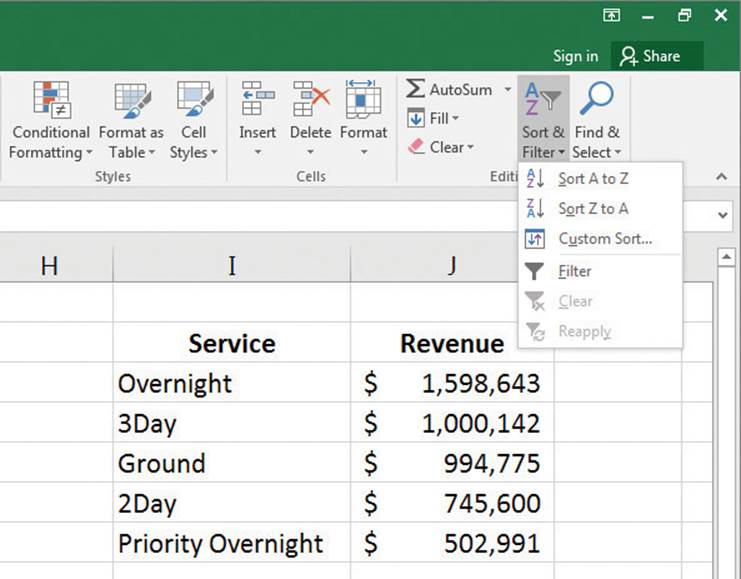
Revenue sorted in descending order
The Sort Smallest To Largest and Sort Largest To Smallest options let you sort rows in a worksheet quickly, but you can use them only to sort the worksheet based on the contents of one column, even though you might want to sort by two columns. For example, you might want to order the worksheet rows by service category and then by total so that you can tell which service categories are used most frequently.
Sort a list of data by more than one column
You can sort rows in a worksheet by the contents of more than one column by using the Sort dialog box, in which you can pick any number of columns to use as sort criteria and choose whether to sort the rows in ascending or descending order. If you want to create two similar rules, perhaps changing just the field to which the rules are applied, you can create a rule for one field, copy it within the Sort dialog box, and change the field name.
If your data cells have fill colors applied to them, perhaps representing cells with values you want your colleagues to notice, you can sort your list of data by using those colors. In addition, you can create more detailed sorting rules, change the order in which rules are applied, and edit and delete rules by using the controls in the Sort dialog box.
Use the Sort dialog box to create detailed sorting rules
To sort worksheet data based on values in a single column
1. Click a cell in the column that contains the data by which you want to sort.
2. On the Home tab of the ribbon, in the Editing group, click the Sort & Filter button to display a menu of sorting and filtering choices.
3. Click Sort A to Z to sort the data in ascending order.
Or
Click Sort Z to A to sort the data in descending order.
To sort worksheet data based on values in multiple columns
1. Click a cell in the list of data you want to sort.
2. On the Sort & Filter menu, click Custom Sort.
3. If necessary, select the My data has headers check box.
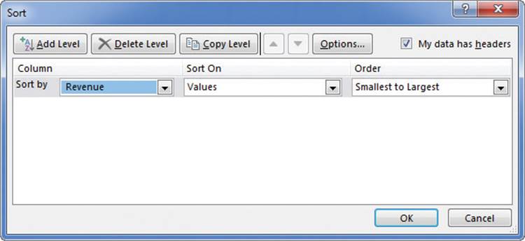
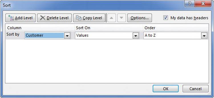
4. In the Sort by list, select the first field; in the Sort On list, select the option by which you want to sort the data (Values, Cell Color, Font Color, or Cell Icon). Then, in the Order list, select an order for the sort operation.
You can create up to 64 sorting levels in Excel 2016
5. Click the Add Level button.
6. In the Then by list, create another rule by using the techniques described in step 4.
7. When you are done creating sort levels, click OK to sort the values.
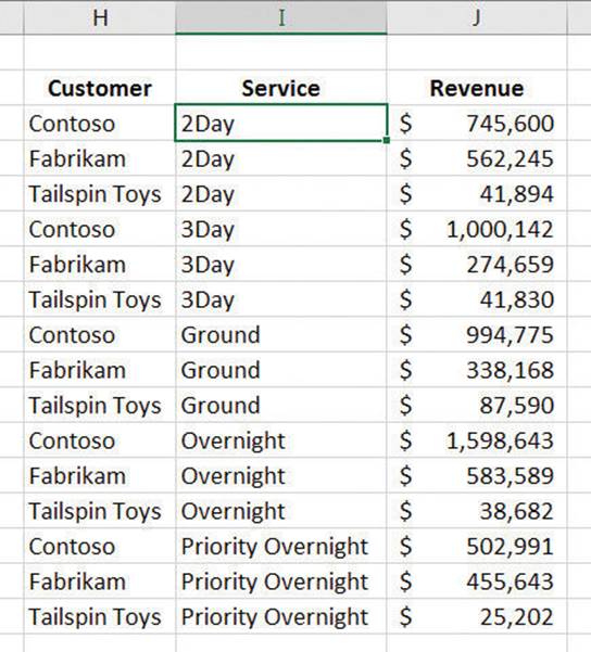
A list of data that has had sorting rules applied to it
To sort by cell color
1. Select a cell in the list of data.
2. On the Sort & Filter menu, click Custom Sort.
3. If necessary, select the My data has headers check box.
4. In the Sort by list, select the field by which you want to sort.
5. In the Sort On list, select Cell Color.
6. In the Order list, select the cell color on which you want to sort.
7. In the last list box, select the position you want for the color you identified (On Top or On Bottom).
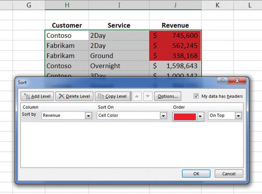
Sort lists of data by using cell fill colors as a criterion
8. When you are done creating sorting rules, click OK to sort the values.
To copy a sorting level
1. Select a cell in the list of data.
2. On the Sort & Filter menu, click Custom Sort.
3. Select the sorting level you want to copy.
4. Click the Copy Level button, and edit the rule as needed.
5. Click OK.
To move a sorting rule up or down in priority
1. On the Sort & Filter menu, click Custom Sort.
2. Select the sorting rule you want to move.
3. Click the Move Up button to move the rule up in the order.
Or
Click the Move Down button to move the rule down in the order.
4. Click OK.
To delete a sorting rule
1. On the Sort & Filter menu, click Custom Sort.
2. Select the sorting level you want to delete.
3. Click the Delete Level button.
4. Click OK.
Sort data by using custom lists
The default setting for Excel is to sort numbers according to their values and to sort words in alphabetical order, but that pattern doesn’t work for some sets of values. One example in which sorting a list of values in alphabetical order would yield incorrect results is the months of the year. In an “alphabetical” calendar, April is the first month and September is the last! Fortunately, Excel recognizes a number of special lists, such as days of the week and months of the year. You can have Excel sort the contents of a worksheet based on values in a known list; if needed, you can create your own list of values. For example, the default lists of weekdays in Excel start with Sunday. If you keep your business records based on a Monday-Sunday week, you can create a new list with Monday as the first day and Sunday as the last.
You can create a new custom list by using controls that are reached through the Excel Options dialog box, which gives you the choice of entering the values yourself or importing them from a cell range in your workbook.
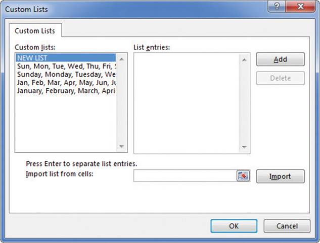
Manage your lists by using the Custom Lists dialog box
![]() Tip
Tip
Another benefit of creating a custom list is that dragging the fill handle of a list cell that contains a value causes Excel to extend the series for you. For example, if you create the list Spring, Summer, Fall, Winter, and then enter Summer in a cell and drag the cell’s fill handle, Excel extends the series as Fall, Winter, Spring, Summer, Fall, and so on.
To define a custom list by entering its values
1. On the File tab, click Options.
2. In the Excel Options dialog box, click the Advanced category.
3. Scroll down to the General area, and then click the Edit Custom Lists button.
4. In the Custom Lists dialog box, enter a list of items in the List entries area.
5. Click Add.
6. Click OK, and then click OK to close the Excel Options dialog box.
To define a custom list by copying values from a worksheet
1. Select the cells that contain the values for your custom list.
2. In the Excel Options dialog box, click the Advanced category.
3. Scroll down to the General area, and click the Edit Custom Lists button.
4. In the Custom Lists dialog box, click the Import button.
5. Click OK, and then click OK to close the Excel Options dialog box.
To sort worksheet data by using a custom list
1. Click a cell in the list of data you want to sort.
2. On the Home tab, click the Sort & Filter button, and then click Custom Sort.
3. If necessary, select the My data has headers check box.
4. In the Sort by list, select the field that contains the data by which you want to sort.
5. If necessary, in the Sort On list, select Values.
6. In the Order list, select Custom List.
7. In the Custom Lists dialog box, select the list you want to use.
8. Click OK.
Organize data into levels
After you have sorted the rows in an Excel worksheet or entered the data so that it doesn’t need to be sorted, you can have Excel calculate subtotals (totals for a portion of the data). In a worksheet with sales data for three different product categories, for example, you can sort the products by category, select all the cells that contain data, and then open the Subtotal dialog box.
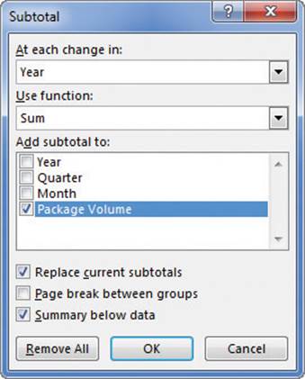
Apply subtotals to data by using the Subtotal dialog box
In the Subtotal dialog box, you can choose the column on which to base your subtotals (such as every change of value in the Week column), the summary calculation you want to perform, and the column or columns with values to be summarized. After you define your subtotals, they appear in your worksheet.
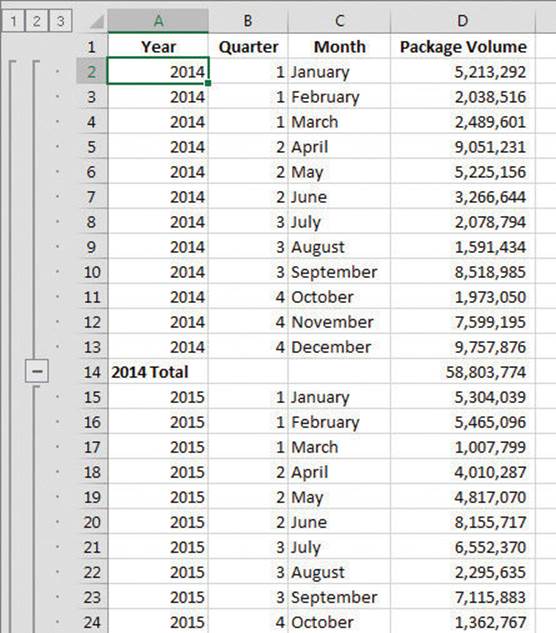
A list of data with Subtotal outlining applied
When you add subtotals to a worksheet, Excel also defines groups based on the rows used to calculate a subtotal. The groupings form an outline of your worksheet based on the criteria you used to create the subtotals. For example, all the rows representing months in the year 2014 could be in one group, rows representing months in 2015 in another, and so on. The outline area at the left of your worksheet holds controls you can use to hide or display groups of rows in your worksheet.
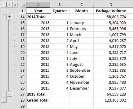
A list of data with details for the year 2014 hidden
When you hide a group of rows, the button displayed next to the group changes to a Show Detail button (the button with the plus sign). Clicking a group’s Show Detail button restores the rows in the group to the worksheet.
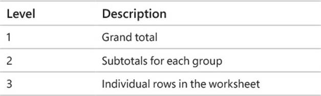
The level buttons are the other buttons in the outline area of a worksheet with subtotals. Each button represents a level of organization in a worksheet; clicking a level button hides all levels of detail below that of the button you clicked. The following table describes the data contained at each level of a worksheet with three levels of organization.
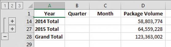
A list of data with details hidden at level 2
If you want, you can add levels of detail to the outline that Excel creates. For example, you might want to be able to hide revenues from January and February, which you know are traditionally strong months. You can also delete any groupings you no longer need, or remove subtotals and outlining entirely.
![]() Tip
Tip
If you want to remove all subtotals from a worksheet, open the Subtotal dialog box, and click the Remove All button.
To organize data into levels
1. Click a cell in the group of data you want to organize.
2. On the Data tab of the ribbon, in the Outline group, click the Subtotal button.
3. In the Subtotal dialog box, in the At each change in list, select the field that controls when subtotals appear.
4. In the Use function list, select the summary function you want to use for each subtotal.
5. In the Add subtotal to group, select the check box next to any field you want to summarize.
6. Click OK.
To show or hide detail in a list with a subtotal summary
1. Do either of the following:
• Click a Hide Detail control to hide a level of detail.
• Click a Show Detail control to show a level of detail.
To create a custom group in a list that has a subtotal summary
1. Select the rows you want to include in the group.
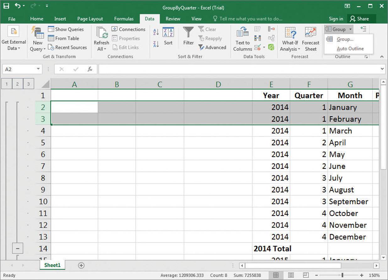
A data list with rows selected to create a custom group
2. Click the Group button.
To remove a custom group in a list that has a subtotal summary
1. Select the rows you want to remove from the group.
2. Click the Ungroup button.
To remove subtotals from a data list
1. Click any cell in the list.
2. Click the Subtotal button.
3. In the Subtotal dialog box, click Remove All.
Look up information in a worksheet
Whenever you create a worksheet that holds information about a list of distinct items, such as products offered for sale by a company, you should ensure that at least one column in the list contains a unique value that distinguishes that row (and the item the row represents) from every other row in the list. Assigning each row a column that contains a unique value means that you can associate data in one list with data in another list. For example, if you assign every customer a unique identification number, you can store a customer’s contact information in one worksheet and all orders for that customer in another worksheet. You can then associate the customer’s orders and contact information without writing the contact information in a worksheet every time the customer places an order.
In technical terms, the column that contains a unique value for each row is known as the primary key column. When you look up information in an Excel worksheet, it is very useful to position the primary key column as the first column in your list of data.
If you know an item’s primary key value, it’s no trouble to look through a list of 20 or 30 items to find it. If, however, you have a list of many thousands of items, looking through the list to find one would take quite a bit of time. Instead, you can use the VLOOKUP function to find the value you want.
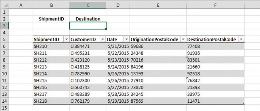
An Excel table for use with VLOOKUP
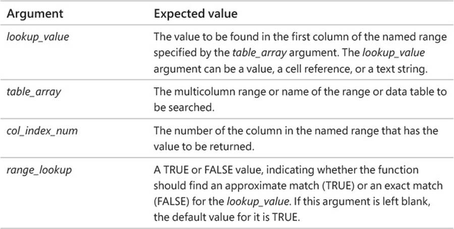
The VLOOKUP function finds a value in the leftmost column of a named range, such as a table, and then returns the value from the specified cell to the right of the cell with the found value. A properly formed VLOOKUP function has four arguments (data that is passed to the function), as shown in the following definition: =VLOOKUP(lookup_value, table_array, col_index_num, range_lookup).
The following table summarizes the values Excel expects for each of these arguments.
![]() Important
Important
When range_lookup is left blank or set to TRUE, for VLOOKUP to work properly, the rows in the named range specified in the table_array argument must be sorted in ascending order based on the values in the leftmost column of the named range.
The VLOOKUP function works a bit differently depending on whether the range_lookup argument is set to TRUE or FALSE. The following list summarizes how the function works based on the value of range_lookup:
![]() If the range_lookup argument is left blank or set to TRUE, and VLOOKUP doesn’t find an exact match for lookup_value, the function returns the largest value that is less than lookup_value.
If the range_lookup argument is left blank or set to TRUE, and VLOOKUP doesn’t find an exact match for lookup_value, the function returns the largest value that is less than lookup_value.
![]() If the range_lookup argument is left blank or set to TRUE, and lookup_value is smaller than the smallest value in the named range, an #N/A error is returned.
If the range_lookup argument is left blank or set to TRUE, and lookup_value is smaller than the smallest value in the named range, an #N/A error is returned.
![]() If the range_lookup argument is left blank or set to TRUE, and lookup_value is larger than all values in the named range, the largest value in the named range is returned.
If the range_lookup argument is left blank or set to TRUE, and lookup_value is larger than all values in the named range, the largest value in the named range is returned.
![]() If the range_lookup argument is set to FALSE, and VLOOKUP doesn’t find an exact match for lookup_value, the function returns an #N/A error.
If the range_lookup argument is set to FALSE, and VLOOKUP doesn’t find an exact match for lookup_value, the function returns an #N/A error.
As an example of a VLOOKUP function, consider the following data, which shows an Excel table with its headers in row 2 and the first column in column B of the worksheet.
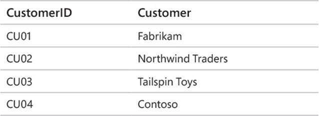
If the =VLOOKUP (E3, B3:C6, 2, FALSE) formula is used, when you enter CU03 in cell E3 and press Enter, the VLOOKUP function searches the first column of the table, finds an exact match, and returns the value Tailspin Toys to cell F3.
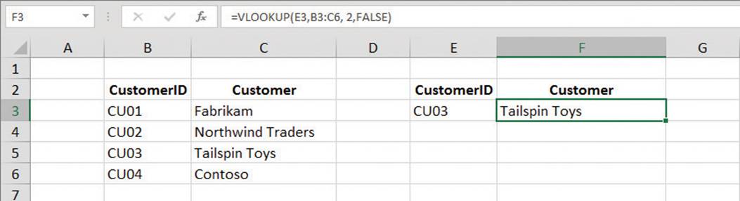
A VLOOKUP formula that looks up a customer name when a customer ID is provided
![]() Tip
Tip
The related HLOOKUP function matches a value in a column of the first row of a table and returns the value in the specified row number of the same column. The letter H in the HLOOKUP function name refers to the horizontal layout of the data, just as the V in the VLOOKUP function name refers to the data’s vertical layout. For more information on using the HLOOKUP function, click the Excel Help button, enter HLOOKUP in the search terms box, and then click Search.
![]() Important
Important
Be sure to give the cell in which you type the VLOOKUP formula the same format as the data you want the formula to display. For example, if you create a VLOOKUP formula in cell G14 that finds a date, you must apply a date cell format to cell G14 for the result of the formula to display properly.
To look up worksheet values by using VLOOKUP
1. Ensure that the data list includes a unique value in each cell of the leftmost column and that the values are sorted in ascending order.
2. In the cell where you want to enter the VLOOKUP formula, enter a formula of the form =VLOOKUP(lookup_value, table_array, col_index_num, range_lookup).
3. Enter TRUE for the range_lookup argument to allow an approximate match.
Or
Enter FALSE for the range_lookup argument to require an exact match.
4. Enter a lookup value in the cell named in the VLOOKUP formula’s first argument, and press Enter.
Skills review
In this chapter, you learned how to:
![]() Sort worksheet data
Sort worksheet data
![]() Sort data by using custom lists
Sort data by using custom lists
![]() Organize data into levels
Organize data into levels
![]() Look up information in a worksheet
Look up information in a worksheet
 Practice tasks
The practice files for these tasks are located in the Excel2016SBS\Ch06 folder. You can save the results of the tasks in the same folder.
Sort worksheet data
Open the SortData workbook in Excel, and then perform the following tasks:
1. Sort the data in the list in ascending order based on the values in the Revenue column.
2. Sort the data in the list in descending order based on the values in the Revenue column.
3. Sort the data in the list in ascending order based on a two-level sort where the first sorting level is the Customer column and the second is the Season column.
4. Change the order of the fields in the previous sort so that the first criterion is the Season column and the second is the Customer column.
5. Sort the data so that the cells in the Revenue column that have a red fill color are at the top of the list.
Sort data by using custom lists
Open the SortCustomData workbook in Excel, and then perform the following tasks:
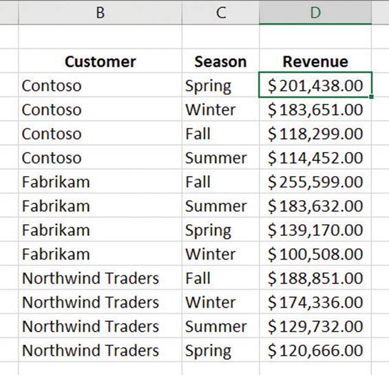
1. Create a custom list by using the values in cells G4:G7.
2. Sort the data in the cell range B3:D14 by the values in the Season column based on the custom list you just created.
3. Create a two-level sort by using the values in the Customer column, in ascending order, as the first criterion, and the custom list-based sort for the Season column as the second.
Organize data into levels
Open the OrganizeData workbook in Excel, and then perform the following tasks:
1. Outline the data list in cells A1:D25 to find the subtotal for each year.
2. Hide the details of rows for the year 2015.
3. Create a new group consisting of the rows showing data for June and July 2014.
4. Hide the details of the group you just created.
5. Show the details of all months for the year 2015.
6. Remove the subtotal outline from the entire data list.
Look up information in a worksheet
Open the LookupData workbook in Excel, and then perform the following tasks:
1. Sort the values in the first table column in ascending order.
2. In cell C3, create a formula that finds the CustomerID value for a ShipmentID entered into cell B3.
3. Edit the formula so that it finds the DestinationPostalCode value for the same package.
All materials on the site are licensed Creative Commons Attribution-Sharealike 3.0 Unported CC BY-SA 3.0 & GNU Free Documentation License (GFDL)
If you are the copyright holder of any material contained on our site and intend to remove it, please contact our site administrator for approval.
© 2016-2026 All site design rights belong to S.Y.A.