Microsoft Excel 2016 Step by Step (2015)
Part 2: Analyze and present data
7. Combine data from multiple sources
In this chapter
![]() Use workbooks as templates for other workbooks
Use workbooks as templates for other workbooks
![]() Link to data in other worksheets and workbooks
Link to data in other worksheets and workbooks
![]() Consolidate multiple sets of data into a single workbook
Consolidate multiple sets of data into a single workbook
Practice files
For this chapter, use the practice files from the Excel2016SBS\Ch07 folder. For practice file download instructions, see the introduction.
Excel 2016 gives you a wide range of tools with which to format, summarize, and present your data. After you have created a workbook to hold data about a particular subject, you can create as many worksheets as you need to make that data easier to find within your workbook. To ensure that every year’s workbook has a similar appearance, you can create a workbook with the characteristics you want, and save it as a pattern, or template, for similar workbooks you will create in the future.
A consequence of organizing your data into different workbooks and worksheets is that you need ways to manage, combine, and summarize data from more than one Excel document. You can always copy data from one worksheet to another, but if the original value were to change, that change would not be reflected in the cell range to which you copied the data. Rather than remembering which cells you need to update when a value changes, you can create a link to the original cell. That way, Excel will update the value for you whenever you open the workbook. If multiple worksheets hold related values, you can use links to summarize those values in a single worksheet.
This chapter guides you through procedures related to using a workbook as a template for other workbooks, linking to data in other workbooks, and consolidating multiple sets of data into a single workbook.
Use workbooks as templates for other workbooks
After you decide on the type of data you want to store in a workbook and what that workbook should look like, you probably want to be able to create similar workbooks without adding all of the formatting and formulas again. For example, you might have established a design for your monthly sales-tracking workbook.
When you have settled on a design for your workbooks, you can save one of the workbooks as a template for similar workbooks you will create in the future. You can leave the workbook’s labels to aid in data entry, but you should remove any existing data from a workbook that you save as a template, both to avoid data entry errors and to remove any confusion as to whether the workbook is a template. You can also remove any worksheets you and your colleagues won’t need by right-clicking the tab of an unneeded worksheet and, on the shortcut menu that appears, clicking Delete.
![]() Tip
Tip
You can also save your Excel 2016 workbook either as an Excel 97-2003 template (.xlt) or as a macro-enabled Excel 2016 workbook template (.xltm). For information about using macros in Excel 2016 workbooks, see Chapter 12, “Automate repetitive tasks by using macros.”
After you save a workbook as a template, you can use it as a model for new workbooks.
![]() Important
Important
Be sure to save your Excel template file in the Custom Office Templates folder so it’s available for you to use later.
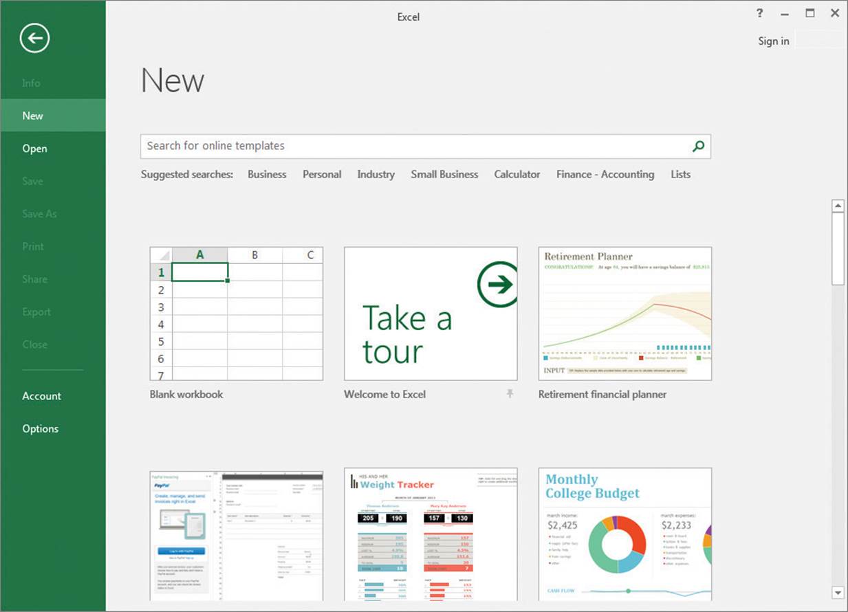
The Backstage view displays available Excel workbook templates
When you create a new workbook by using the tools found in the Backstage view, the New page displays the blank workbook template, built-in templates, a search box you can use to locate helpful templates on Office.com, and a set of sample search terms.
From the list of available templates, you can click the template you want to use as the model for your workbook. Excel creates a new workbook (an .xlsx workbook file, not an .xltx template file) with the template’s formatting and contents in place.
In addition to creating a workbook template, you can add a worksheet based on a worksheet template to your workbook by using the Insert dialog box.
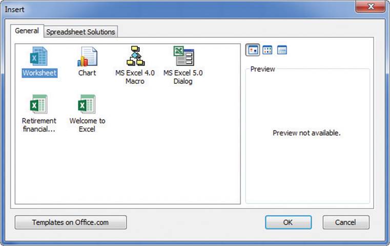
Add specific worksheet types by using the Insert dialog box
The Insert dialog box splits its contents into two tabs. The General tab contains icons you can click to insert a blank worksheet, a chart sheet, and any worksheet templates available to you.
![]() Tip
Tip
The other two options on the General tab, MS Excel 4.0 Macro and MS Excel 5.0 Dialog, are there to help users include solutions built in earlier versions of Excel into Excel 2016.
The Spreadsheet Solutions tab contains a set of useful templates for a variety of financial and personal tasks. If you want to create a worksheet template, as opposed to a workbook template, delete all but one worksheet from your file and save it as a template.
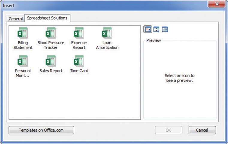
Create useful worksheets from the Spreadsheet Solutions tab
To create a workbook by using an existing template
1. Click the File tab to display the Backstage view.
2. Click New.
3. If necessary, enter a search term in the Search for online templates box and press Enter.
4. Click the template you want to use.
5. Click Create.
To insert a worksheet template into a workbook
1. Right-click any sheet tab and, on the shortcut menu that appears, click Insert.
2. In the Insert dialog box, click the tab that contains the worksheet template you want to use.
3. Click the worksheet template.
4. Click OK.
To save a workbook as a template
1. Create the workbook you want to save as a template.
2. In the Backstage view, click Save As.
3. Click Browse.
4. Click the Save as type arrow, and then click Excel Template.
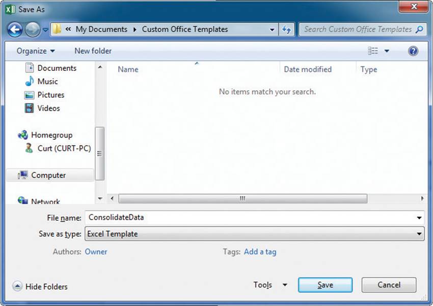
Click the Excel Template file type to use your file as a pattern for other workbooks
5. In the File name box, enter a name for the template workbook.
6. Click Save.
To save a workbook as a macro-enabled template
1. Create the workbook you want to save as a macro-enabled template.
2. In the Backstage view, click Save As.
3. Click Browse.
4. Click the Save as type arrow, and then click Excel Macro-Enabled Template.
5. In the File name box, enter a name for the template workbook.
6. Click Save.
Link to data in other worksheets and workbooks
Copying and pasting data from one workbook to another is a quick and easy way to gather related data in one place, but there is a substantial limitation: If the data from the original cell changes, the change is not reflected in the cell to which the data was copied. In other words, copying and pasting a cell’s contents doesn’t create a relationship between the original cell and the target cell.
You can ensure that the data in the target cell reflects any changes in the original cell by creating a link between the two cells. Instead of entering a value into the target cell by typing or pasting, you create a formula that identifies the source from which Excel derives the target cell’s value, and that updates the value when it changes in the source cell.
You can link to a cell in another workbook by starting to create your formula, displaying the worksheet that contains the value you want to use, and then selecting the cell or cell range you want to include in the calculation. When you press Enter and switch back to the workbook with the target cell, the value in the formula bar shows that Excel has filled in the formula with a reference to the cell you clicked.
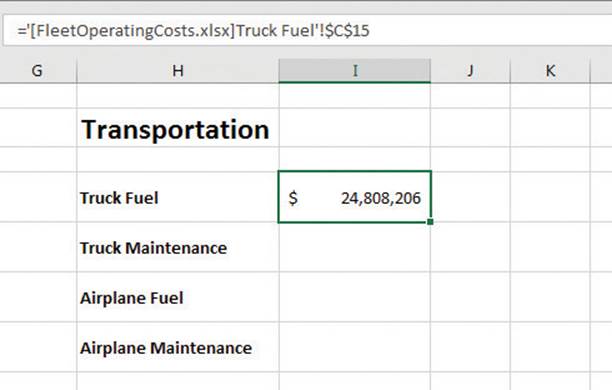
A 3-D cell reference to another workbook
The reference =‘[FleetOperatingCosts.xlsx]Truck Fuel’!$C$15 gives three pieces of information: the workbook, the worksheet, and the cell you linked to in the worksheet. The first element of the reference, the name of the workbook, is enclosed in brackets; the end of the second element (the worksheet) is marked with an exclamation point; and the third element, the cell reference, has a dollar sign before both the row and the column identifier. The single quotes around the workbook name and worksheet name are there to allow for the space in the Truck Fuel worksheet’s name. This type of reference is known as a 3-D reference, reflecting the three dimensions (workbook, worksheet, and cell range) that you need to point to a group of cells in another workbook.
![]() Tip
Tip
For references to cells in the same workbook, the workbook information is omitted. Likewise, references to cells in the same worksheet don’t use a worksheet identifier.
You can also link to cells in an Excel table. Such links include the workbook name, worksheet name, the name of the Excel table, and row and column references of the cell to which you’ve linked. Creating a link to the Cost column’s cell in a table’s Totals row, for example, results in a reference such as =‘FleetOperatingCosts.xlsx’!Truck Maintenance[[#Totals],[Cost]].
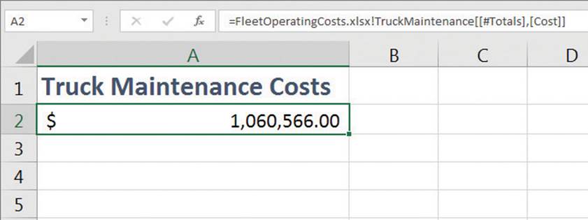
Link to an Excel table value in another workbook
![]() Important
Important
Hiding or displaying a table’s Totals row affects any links to a cell in that row. Hiding the Totals row causes references to that row to display a #REF! error message.
Whenever you open a workbook containing a link to another document, Excel tries to update the information in linked cells. If the app can’t find the source, as would happen if a workbook or worksheet is deleted or renamed, an alert box appears to indicate that there is a broken link. From within that alert box, you can access tools to fix the link reference.

A dialog box that indicates that the workbook just opened contains one or more broken links
If you enter a link into a cell and you make an error, a #REF! error message appears in the cell that contains the link.
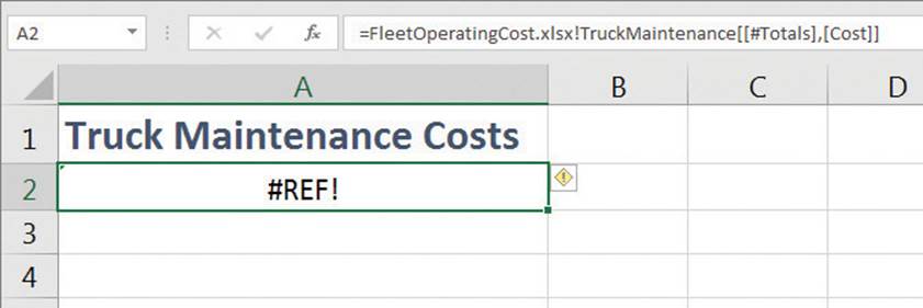
Cells that contain incorrect links display a #REF! error
To fix the link, click the cell, delete its contents, and then either retype the link or create it with the point-and-click method described in the procedures for this topic. Excel might also display errors if the cell values in the worksheet cells you link to change in value and cause errors such as DIV/0! (divide by zero).
![]() Tip
Tip
Excel tracks workbook changes, such as when you change a workbook’s name, very well. Unless you delete a worksheet or workbook, or move a workbook to a new folder, odds are good that Excel can update your link references automatically to reflect the change.
To create a link to a cell or cell range on another worksheet
1. Start creating a formula that will include a value from a cell or cell range on another worksheet.
2. Click the sheet tab of the worksheet with the cell or cell range you want to include in the formula.
3. Select the cell or cells to include in the formula.
4. Press Enter.
To create a link to a cell or cell range in another workbook
1. Open the workbook where you want to create the formula that references an external cell or cell range.
2. Open the workbook that contains the cell or cell range you want to include in your formula.
3. Switch back to the original workbook and start creating a formula that will include a value from a cell or cell range in the other workbook.
4. Display the workbook that contains the cell or cell range you want to include in the formula.
5. Click the sheet tab of the worksheet with the cell or cell range you want to include in the formula.
6. Select the cell or cells to include in the formula.
7. Press Enter.
To create a link to cells in an Excel table
1. Start creating a formula that will include a value from cells in an Excel table.
2. Click the sheet tab of the worksheet with the Excel table that contains the cells you want to include in the formula.
3. Select the cell or cells to include in the formula.
4. Press Enter.
To open the source of a linked value
1. Open a workbook that contains a link to an external cell or cell range.
2. On the Data tab of the ribbon, in the Connections group, click the Edit Links button.
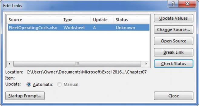
Manage workbook links by using the Edit Links dialog box
3. In the Edit Links dialog box, click the link you want to work with.
4. Click the Open Source button.
To fix a link that returns an error because it references the wrong workbook
1. Click the Edit Links button.
2. In the Edit Links dialog box, click the link that returns an error.
3. Click Change Source.
4. Click the workbook that contains the correct source value.
5. If the Select Sheet dialog box appears, click the worksheet that contains the correct source value, and click OK.
6. Click Close.
To break a link
1. In a workbook that contains a link to a cell on another worksheet or in another workbook, click the Edit Links button.
2. In the Edit Links dialog box, click the link you want to edit.
3. Click the Break Link button. When prompted, click Break Links to confirm that you want to break the link.
4. Click Close.
![]() Tip
Tip
If you can’t easily fix a link that returns an error, the best choice is often to delete the link from the formula and re-create it.
Consolidate multiple sets of data into a single workbook
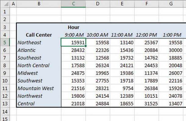
When you create a series of worksheets that contain similar data, perhaps by using a template, you build a consistent set of workbooks in which data is stored in a predictable place. For example, consider a workbook template used to track the number of calls received from 9:00 A.M. to 10:00 P.M.
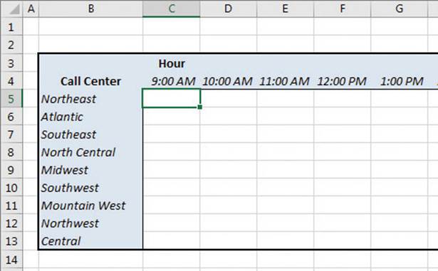
Consolidation targets should have labels but no data
Using links to bring data from one worksheet to another gives you a great deal of power to combine data from several sources into a single resource. For example, you can create a worksheet that lists the number of calls you receive during specific hours of the day, use links to draw the values from the worksheets in which the call counts were recorded, and then create a formula to perform calculations on the data. However, for large worksheets with hundreds of cells filled with data, creating links from every cell is a time-consuming process. Also, to calculate a sum or an average for the data, you would need to include links to cells in every workbook.
Fortunately, there is an easier way to combine data from multiple worksheets in a single worksheet. By using this process, called data consolidation, you can define ranges of cells from multiple worksheets and have Excel summarize the data. You define these ranges in the Consolidate dialog box.
![]() Important
Important
To consolidate data, every range included in the consolidation must be of the same shape and size.
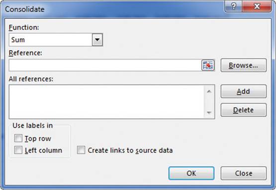
Summarize data sets of the same shape by using consolidation
Cells that are in the same relative position in the ranges have their contents summarized together. When you consolidate the ranges, the cell in the upper-left corner of one range is added to the cell in the upper-left corner of every other range, even if those ranges are in different areas of the worksheet. After you choose the ranges to be used in your summary, you can choose the calculation to perform on the data. Excel sums the data by default, but you can select other functions to summarize the data.
![]() Important
Important
You can define only one data consolidation summary per workbook.
To consolidate cell ranges from multiple worksheets or workbooks
1. Open the workbook into which you want to consolidate your data and the workbooks supplying the data for the consolidated range.
2. In the workbook into which you want to consolidate your data, on the Data tab, in the Data Tools group, click Consolidate.
3. In the Consolidate dialog box, click the Collapse Dialog button at the right edge of the Reference field to collapse the dialog box.
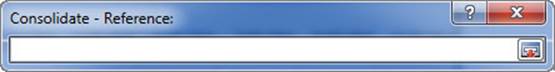
Clicking the Collapse Dialog button minimizes the Consolidate dialog box
4. On the View tab, in the Window group, click Switch Windows and then, in the list, click the first workbook that contains data you want to include.
5. Select the cell range, click the Expand Dialog button to restore the Consolidate dialog box to its full size, and click Add to add the selected range to the All references pane.
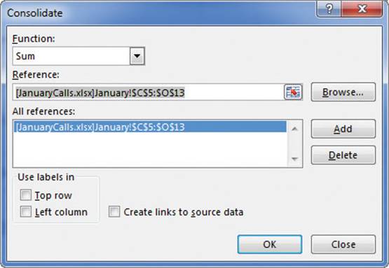
Add data ranges to create a consolidation range
6. Repeat steps 3 through 5 to add additional ranges to the consolidation.
7. If you want to change the summary function, click the Function arrow in the Consolidate dialog box and select a new function from the list.
8. Click OK.
Skills review
In this chapter, you learned how to:
![]() Use workbooks as templates for other workbooks
Use workbooks as templates for other workbooks
![]() Link to data in other worksheets and workbooks
Link to data in other worksheets and workbooks
![]() Consolidate multiple sets of data into a single workbook
Consolidate multiple sets of data into a single workbook
 Practice tasks
The practice files for these tasks are located in the Excel2016SBS\Ch07 folder. You can save the results of the tasks in the same folder.
Use workbooks as templates for other workbooks
Open the CreateTemplate workbook in Excel, and then perform the following tasks:
1. Add a worksheet based on an existing template, such as the Sales Report template, to the workbook.
2. Save the new workbook as a template and close it.
3. In the Backstage view, click New.
4. Create a new workbook based on an existing template.
Link to data in other worksheets and workbooks
Open the CreateDataLinks and FleetOperatingCosts workbooks in Excel, and then perform the following tasks:
1. In the CreateDataLinks workbook, create links to the FleetOperatingCosts workbook that copy truck fuel, truck maintenance, airplane fuel, and airplane maintenance costs to the appropriate cells in column I on Sheet1 of the CreateDataLinks workbook.
2. Close the FleetOperatingCosts workbook.
3. View the links in the CreateDataLinks workbook and show the source for one of the links.
4. Break the link to the airplane fuel source data cell.
Consolidate multiple sets of data into a single workbook
Open the ConsolidateData, JanuaryCalls, and FebruaryCalls workbooks in Excel, and then perform the following tasks:
1. In the ConsolidateData workbook, create a consolidation target by using cells C5:O13.
2. Add call data from the JanuaryCalls workbook’s cell range C5:O13 as a consolidation range.
3. Add call data from the FebruaryCalls workbook’s cell range C5:O13 as a consolidation range.
4. Click OK.
A completed consolidation summary
All materials on the site are licensed Creative Commons Attribution-Sharealike 3.0 Unported CC BY-SA 3.0 & GNU Free Documentation License (GFDL)
If you are the copyright holder of any material contained on our site and intend to remove it, please contact our site administrator for approval.
© 2016-2026 All site design rights belong to S.Y.A.