Microsoft Excel 2016 Step by Step (2015)
Part 2: Analyze and present data
8. Analyze alternative data sets
In this chapter
![]() Examine data by using the Quick Analysis Lens
Examine data by using the Quick Analysis Lens
![]() Define an alternative data set
Define an alternative data set
![]() Define multiple alternative data sets
Define multiple alternative data sets
![]() Analyze data by using data tables
Analyze data by using data tables
![]() Vary your data to get a specific result by using Goal Seek
Vary your data to get a specific result by using Goal Seek
![]() Find optimal solutions by using Solver
Find optimal solutions by using Solver
![]() Analyze data by using descriptive statistics
Analyze data by using descriptive statistics
Practice files
For this chapter, use the practice files from the Excel2016SBS\Ch08 folder. For practice file download instructions, see the introduction.
When you store data in an Excel 2016 workbook, you can use that data, either by itself or as part of a calculation, to discover important information about your organization. You can summarize your data quickly by using the Quick Analysis Lens to create charts, calculate totals, or apply conditional formatting.
The data in your worksheets is great for answering “what-if” questions, such as, “How much money would we save if we reduced our labor to 20 percent of our total costs?” You can always save an alternative version of a workbook and create formulas that calculate the effects of your changes, but you can do the same thing in your existing workbooks by defining one or more alternative data sets. You can also create a data table that calculates the effects of changing one or two variables in a formula, find the input values required to generate the result you want, and describe your data statistically.
This chapter guides you through procedures related to examining data by using the Quick Analysis Lens, defining an alternative data set, defining multiple alternative data sets, analyzing data by using data tables, varying data to get a specific result by using Goal Seek, finding optimal solutions by using Solver, and analyzing data by using descriptive statistics.
Examine data by using the Quick Analysis Lens
One useful tool in Excel 2016 is the Quick Analysis Lens, which brings the most commonly used formatting, charting, and summary tools into one convenient location. After you select the data you want to summarize, clicking the Quick Analysis action button displays the tools you can use to analyze your data.
Click the Quick Analysis action button to display analysis tools
![]() Tip
Tip
To display the Quick Analysis toolbar by using a keyboard shortcut, press Ctrl+Q.
The Quick Analysis toolbar makes a wide range of tools available, including the ability to create an Excel table or PivotTable, insert a chart, or add conditional formatting. You can also add total columns and rows to your data range.
Select from several categories of analysis tools
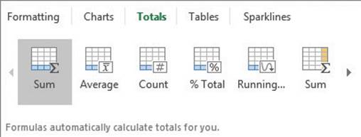
You can use the tools on the Totals tab of the Quick Analysis toolbar to add summary operations to your data. You can add one summary column and one summary row to each data range. If you select a new summary column or row when one exists, Excel displays a confirmation dialog box to verify that you want to replace the existing summary.
To add formatting by using the Quick Analysis Lens
1. Select the cells you want to analyze.
2. Click the Quick Analysis action button.
3. If necessary, click the Formatting tab.
4. Click the button that represents the formatting you want to apply.
To add totals by using the Quick Analysis Lens
1. Select the cells you want to analyze.
2. Click the Quick Analysis action button.
3. If necessary, click the Totals tab.
4. Click the button that represents the total you want to apply.
To add tables by using the Quick Analysis Lens
1. Select the cells you want to analyze.
2. Click the Quick Analysis action button.
3. If necessary, click the Tables tab.
4. Click the button that represents the type of table you want to create.
Define an alternative data set
When you save data in an Excel worksheet, you create a record that reflects the characteristics of an event or object. That data could represent the number of deliveries in an hour on a particular day, the price of a new delivery option, or the percentage of total revenue accounted for by a delivery option. After the data is in place, you can create formulas to generate totals, find averages, and sort the rows in a worksheet based on the contents of one or more columns. However, if you want to perform a what-if analysis or explore the impact that changes in your data would have on any of the calculations in your workbooks, you need to change your data.
The problem with manipulating data that reflects an event or item is that when you change any data to affect a calculation, you run the risk of destroying the original data if you accidentally save your changes. You can avoid ruining your original data by creating a duplicate workbook and making your changes to it, but you can also create an alternative data set, or scenario, within an existing workbook.
When you create a scenario, you give Excel alternative values for a list of cells in a worksheet. You can use the Scenario Manager to add, delete, and edit scenarios.
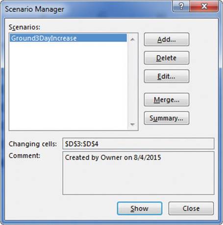
Track and change scenarios by using the Scenario Manager
When you’re ready to add a scenario, you start by providing its name and, if you want, a comment describing the scenario.
![]() Tip
Tip
Adding a comment gives you and your colleagues valuable information about the scenario and your purpose for creating it. Many Excel users create scenarios without comments, but comments are extremely useful when you work on a team or revisit a workbook after several months.
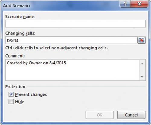
Define a scenario in the Add Scenario dialog box
After you name your scenario, you can define its values.
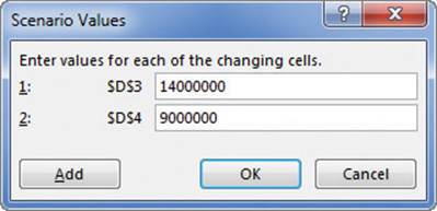
Enter alternative data in the Scenario Values dialog box
After you have created your scenario, clicking the Show button in the Scenario Manager replaces the values in the original worksheet with the alternative values you just defined in the scenario. Any formulas that reference cells with changed values will recalculate their results. You can then remove the scenario by clicking the Undo button on the Quick Access Toolbar.
![]() Important
Important
If you save and close a workbook while a scenario is in effect, those values become the default values for the cells changed by the scenario! You should seriously consider creating a scenario that contains the original values of the cells you change or creating a scenario summary worksheet (a subject covered in the next topic).
The tools available in the Scenario Manager also let you edit your scenarios and delete the ones you no longer need.
To define an alternative data set by creating a scenario
1. On the Data tab, in the Forecast group, click the What-If Analysis button to display a menu of the what-if choices, and then click Scenario Manager.
2. In the Scenario Manager dialog box, click Add.
3. In the Scenario name box, enter a name for the scenario.
4. Click in the Changing cells box, and then select the cells you want to change.
5. Click OK.
6. In the Scenario Values dialog box, enter new values for each of the changing cells.
7. Click OK.
8. Click Close to close the Scenario Manager dialog box.
To display an alternative data set
1. On the What-if Analysis menu, click Scenario Manager.
2. In the Scenario Manager dialog box, click the scenario you want to display.
3. Click Show.
4. If you want to close the Scenario Manager dialog box, click Close.
To edit an alternative data set
1. On the What-If Analysis menu, click Scenario Manager.
2. In the Scenario Manager dialog box, click the scenario you want to edit.
3. Click Edit.
4. In the Edit Scenario dialog box, change the values in the Scenario name, Changing cells, or Comment box.
5. Click OK.
6. In the Scenario Values dialog box, enter new values for each of the changing cells.
7. Click OK.
8. Click Close to close the Scenario Manager dialog box.
To delete an alternative data set
1. On the What-if Analysis menu, click Scenario Manager.
2. In the Scenario Manager dialog box, click the scenario you want to delete.
3. Click Delete.
4. Click Close to close the Scenario Manager dialog box.
Define multiple alternative data sets
One great feature of Excel scenarios is that you’re not limited to creating one alternative data set—you can create as many scenarios as you want and apply them by using the Scenario Manager.
![]() Tip
Tip
If you apply a scenario to a worksheet and then apply another scenario to the same worksheet, both sets of changes appear. If multiple scenarios change the same cell, the cell will contain the value in the most recently applied scenario.
Applying multiple scenarios alters the values in your worksheets. You can see how those changes affect your formulas, but Excel also lets you create a record of your different scenarios by using the Scenario Summary dialog box. From within the dialog box, you can choose the type of summary worksheet you want to create and the cells you want to display in the summary worksheet.
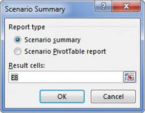
Summarize scenarios by using the Scenario Summary dialog box
![]() Important
Important
Make sure you don’t have any scenarios applied to your workbook when you create the summary worksheet. If you do have an active scenario, Excel will record the scenario’s changed values as the originals, and your summary will be inaccurate.
It’s a good idea to create an “undo” scenario named Normal that holds the original values of the cells you’re going to change before you change them in other scenarios. For example, if you create a scenario that changes the values in three cells, your Normal scenario restores those cells to their original values. That way, even if you accidentally modify your worksheet, you can apply the Normal scenario and not have to reconstruct the worksheet from scratch.
![]() Important
Important
Each scenario can change a maximum of 32 cells, so you might need to create more than one scenario to ensure that you can restore a worksheet.
To apply multiple alternative data sets
1. On the Data tab, in the Forecast group, click the What-If Analysis button to display a menu of the what-if choices, and then click Scenario Manager.
2. In the Scenario Manager dialog box, click the scenario you want to display.
3. Click Show.
4. Repeat steps 2 and 3 for any additional scenarios you want to display.
5. Click Close.
To create a scenario summary worksheet
1. On the What-if Analysis menu, click Scenario Manager.
2. In the Scenario Manager dialog box, click Summary.
3. In the Scenario Summary dialog box, click Scenario summary.
4. Click OK.
Analyze data by using data tables
When you examine business data in Excel, you will often want to discover what the result of a formula would be with different input values. In Excel 2016, you can calculate the results of those changes by using a data table. To create a data table with one variable, you create a worksheet that contains the data required to calculate the variations in the table.
Perform data analysis by changing one variable
![]() Important
Important
You must lay out the data and formulas in a rectangle so the data table you create will appear in the lower-right corner of the cell range you select.
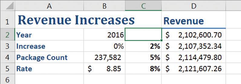
For example, you can put the formula used to summarize the base data in cell D2, the cells with the changing values in the range C3:C5, and the cells to contain the calculations based on those values in D3:D5. Given the layout of this specific worksheet, you would select cells C2:D5, which contain the summary formula, the changing values, and the cells where the new calculations should appear.
After you select the data and the formula, you can use the Data Table dialog box to perform your analysis.
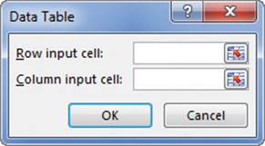
Identify input cells for your data table
To change a single variable, you identify the cell that contains the summary formula’s value that will change in the data table’s cells. In this example, that cell is B3. Because the target cells D3:D5 are laid out as a column, you would identify that range as the column input cell.
![]() Tip
Tip
If your target cells were laid out as a row, you would enter the address of the cell containing the value to be changed in the Row Input Cell box.
When you click OK, Excel fills in the results of the data table, using the replacement values in cells C3:C5 to provide the values for cells D3:D5.
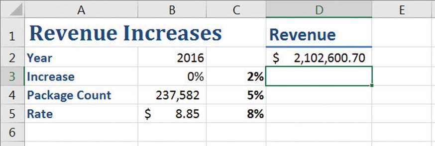
A completed one-variable data table
To create a two-variable data table, you lay your data out with one set of replacement values as row headers and the other set as column headers.
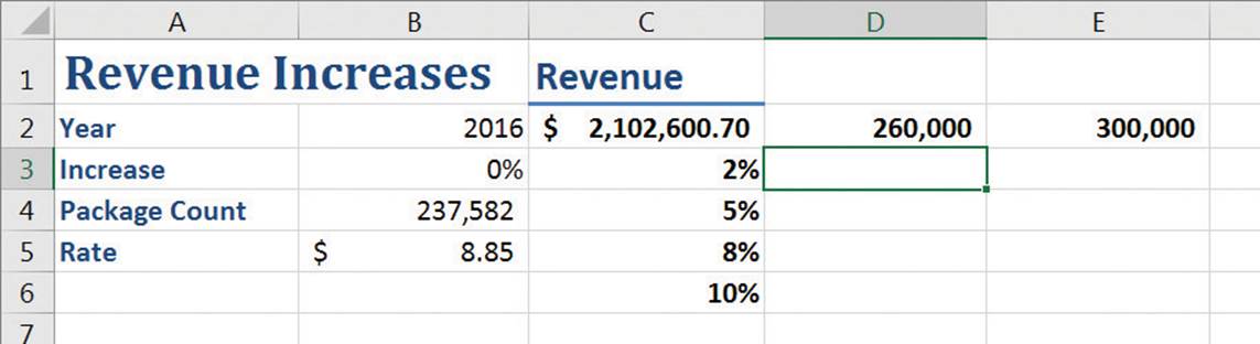
Two-variable data tables replace both row and column values
In this example, you would select the cell range C2:E5 and create the data table. Because you’re creating a two-variable data table, you need to enter cell addresses for both the column input cell and row input cell. The column input cell is B3, which represents the rate increase, and the row input cell is B4, which contains the package count. When you’re done, Excel creates your data table.
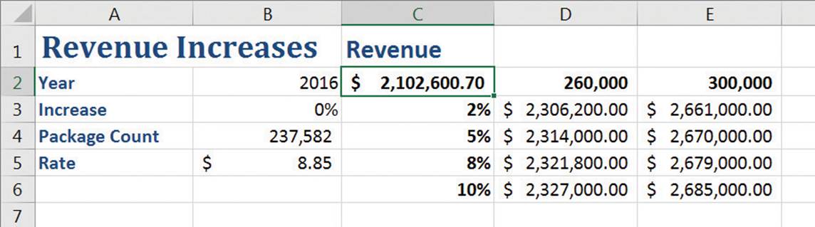
Replacing both row and column values generates multiple outcomes
![]() Tip
Tip
For a two-value data table, the summary formula should be the top-left cell in the range you select before creating the data table.
To create a one-variable data table
1. Create a worksheet with a summary formula, the input values that the summary formula uses to calculate its value, and a series of adjacent cells that contain alternative values for one of the summary formula’s input values.
2. Select the cells representing the summary formula and the changing values, and the cells where the alternative summary formula results should appear.
3. On the Data tab, in the Forecast group, click the What-If Analysis button to display a menu of the what-if choices, and then click Data Table.
4. In the Data Table dialog box, do either of the following:
• If the changing values appear in a row, in the Row input cell box, enter the cell address of the changing value.
• If the changing values appear in a column, in the Column input cell box, enter the cell address of the changing value.
5. Click OK.
To create a two-variable data table
1. Create a worksheet with a summary formula, the input values that the summary formula uses to calculate its value, and two series of adjacent cells (one in a row, one in a column) that contain alternative values for two of the summary formula’s input values.
2. Select the cells representing the summary formula and the changing values, and the cells where the alternative summary formula results should appear.
3. On the What-If Analysis menu, click Data Table.
4. In the Data Table dialog box, in the Row input cell box, enter the cell address of the cell that has alternative values that appear in a worksheet row.
5. In the Column input cell box, enter the cell address of the cell that has alternative values that appear in a worksheet column.
6. Click OK.
Vary your data to get a specific result by using Goal Seek
When you run an organization, you must track how every element performs, both in absolute terms and in relation to other parts of the organization. There are many ways to measure your operations, but one useful technique is to limit the percentage of total costs contributed by a specific item.
As an example, consider a worksheet that contains the actual costs and percentage of total costs for several production input values.
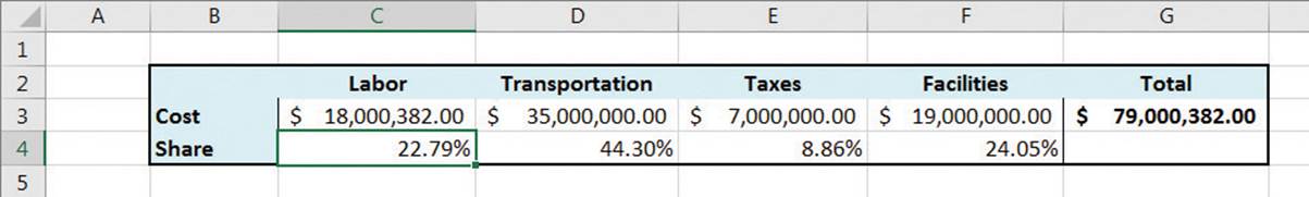
A worksheet that calculates the percentage of total costs for each of four categories
Under the current pricing structure, Labor represents 22.79 percent of the total costs for the product. If you’d prefer that Labor represent no more than 20 percent of total costs, you can change the cost of Labor manually until you find the number you want. Rather than do it manually, though, you can use Goal Seek to have Excel find the solution for you.
When you use Goal Seek, you identify the cell that contains the formula you use to evaluate your data, the target value, and the cell you want to change to generate that target value.
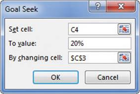
Identify the cell that contains the formula you want to use to generate a target value
Clicking OK tells Excel to find a solution for the goal you set. When Excel finishes its work, the new values appear in the designated cells, and the Goal Seek Status dialog box opens.
![]() Important
Important
If you save a workbook with the results of a Goal Seek calculation in place, you will overwrite the values in your workbook.
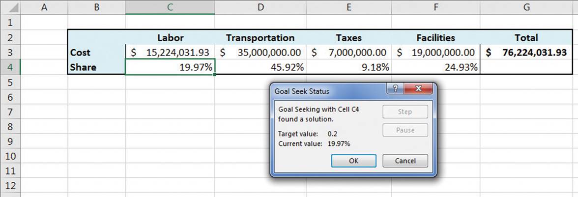
A worksheet where Goal Seek found a solution to a problem
![]() Tip
Tip
Goal Seek finds the closest solution it can without exceeding the target value.
To find a target value by using Goal Seek
1. On the Data tab, in the Forecast group, click the What-If Analysis button, and then click Goal Seek.
2. In the Goal Seek dialog box, in the Set cell box, enter the address of the cell that contains the formula you want to use to produce a specific value.
3. In the To value box, enter the target value for the formula you identified.
4. In the By changing cell box, enter the address of the cell that contains the value you want to vary to produce the result you want.
5. Click OK.
Find optimal solutions by using Solver
Goal Seek is a great tool for finding out how much you need to change a single input value to generate a specific result from a formula, but it’s of no help if you want to find the best mix of several input values. For more complex problems that seek to maximize or minimize results based on several input values and constraints, you need to use Solver.
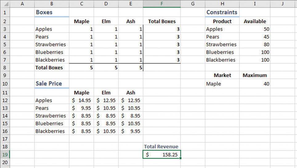
Use Solver to select a product distribution to maximize revenue
![]() Tip
Tip
It helps to spell out every aspect of your problem so that you can identify the cells you want Solver to use in its calculations.
If you performed a complete installation when you installed Excel on your computer, the Solver button will appear on the Data tab in the Analyze group. If not, you can install the Solver add-in from the Add-Ins page of the Excel Options dialog box. After the installation is complete, Solver appears on the Data tab, in the Analyze group, and you can create your model.
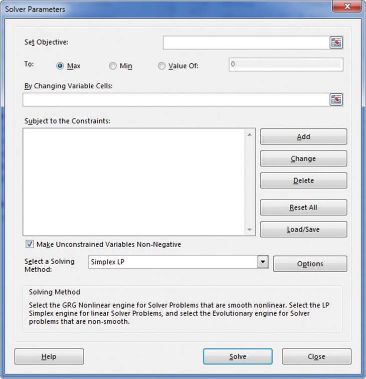
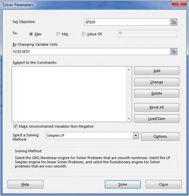
Create a Solver model by using the Solver Parameters dialog box
The first step in setting up your Solver problem is to identify the cell that contains the summary formula you want to establish as your objective, followed by indicating whether you want to minimize the cell’s value, maximize the cell’s value, or make the cell take on a specific value. Next, you select the cells Solver should vary to change the value in the objective cell. You can, if you want, require Solver to find solutions that use only integer values (that is, values that are whole numbers and have no decimal component).
![]() Important
Important
Finding integer-only solutions, or integer programming, is much harder than finding solutions that allow decimal values. It might take Solver several minutes to find a solution or to discover that a solution using just integer values isn’t possible.
Next, you create constraints that will set the limits for the values Solver can use. The best way to set your constraints is to specify them in your worksheet. Basing Solver constraints on worksheet cell values lets you add labels and explanatory text in neighboring cells and change the constraints quickly, without opening the Solver Parameters dialog box.
![]() Tip
Tip
After you run Solver, you can use the commands in the Solver Results dialog box to save the results as changes to your worksheet or create a scenario based on the changed data.
Finally, you need to select the solving method that Solver will use to look for a solution to your problem. There are three options, each of which works best for a specific type of problem:
![]() Simplex LP Used to solve problems where all of the calculations are linear, meaning they don’t involve exponents or other non-linear elements.
Simplex LP Used to solve problems where all of the calculations are linear, meaning they don’t involve exponents or other non-linear elements.
![]() GRG Nonlinear Used to solve problems where the calculations involve exponents or other non-linear mathematical elements.
GRG Nonlinear Used to solve problems where the calculations involve exponents or other non-linear mathematical elements.
![]() Evolutionary Uses genetic algorithms to find a solution. This method is quite complex and can take far longer to run than either of the other two engines, but if neither the Simplex LP or GRG Nonlinear engines can find a solution, the Evolutionary engine might be able to.
Evolutionary Uses genetic algorithms to find a solution. This method is quite complex and can take far longer to run than either of the other two engines, but if neither the Simplex LP or GRG Nonlinear engines can find a solution, the Evolutionary engine might be able to.
![]() Tip
Tip
If you’re using the Simplex LP engine and Solver returns an error immediately, indicating that it can’t find a solution, try using the GRG Nonlinear engine.
To add Solver to the ribbon
1. Click the File tab, and then in the Backstage view, click Options.
2. In the Excel Options dialog box, click the Add-Ins category.
3. If necessary, in the Manage list, click Excel Add-ins. When Excel Add-ins appears in the Manage box, click Go.
4. In the Add-Ins dialog box, select the Solver Add-in check box.
5. Click OK.
To open the Solver Parameters dialog box
1. On the Data tab, in the Analyze group, click Solver.
To identify the objective cell of a model
1. Click Solver.
2. In the Solver Parameters dialog box, click in the Set Objective box.
3. Click the cell that includes the formula you want to optimize.
To specify the type of result your Solver model should return
1. In the Solver Parameters dialog box, do any of the following:
• Select Max to maximize the objective cell’s value.
• Select Min to minimize the objective cell’s value.
• Select Value Of and enter the target value in the box to the right to generate a specific result.
To identify the cells with values that can be changed
1. In the Solver Parameters dialog box, click in the By Changing Variable Cells box.
2. Select the cells you will allow Solver to change to generate a solution.
Identify the cells Solver can change to find a solution
To add a constraint to your Solver model
1. In the Solver Parameters dialog box, click Add.
2. In the Add Constraint dialog box, in the Cell Reference box, identify the cells to which you want to apply the constraint.
3. In the middle list box, click the arrow, and then click the type of constraint you want to apply.
4. Click in the Constraint box and do either of the following:
• Enter the address of the cell that contains the constraint’s comparison value.
• Select the cell that contains the constraint’s comparison value.
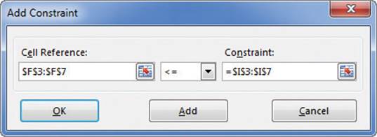
Add constraints to reflect the specified circumstances of your business
5. Click Add to create a new constraint.
Or
Click OK to close the Add Constraint dialog box.
To require a value to be a binary number (0 or 1)
1. In the Add Constraint dialog box, in the Cell Reference box, identify the cells to which you want to apply the constraint.
2. In the middle list box, click the arrow, and then click bin.
3. Click OK.
To require a value to be an integer
1. In the Add Constraint dialog box, in the Cell Reference box, identify the cells to which you want to apply the constraint.
2. In the middle list box, click the arrow, and then click int.
3. Click OK.
To edit a constraint
1. In the Solver Parameters dialog box, click the constraint you want to edit.
2. Click Change.
3. In the Change Constraint dialog box, in the Cell Reference box, identify the cells to which you want to apply the constraint.
4. In the middle list box, click the arrow, and then click the type of constraint you want to apply.
5. Click in the Constraint box and do either of the following:
• Enter the address of the cell that contains the constraint’s comparison value.
• Select the cell that contains the constraint’s comparison value.
6. Click OK.
To delete a constraint
1. In the Solver Parameters dialog box, click the constraint you want to delete.
2. Click Delete.
To require changing cells to contain non-negative values
1. In the Solver Parameters dialog box, select the Make Unconstrained Variables Non-Negative check box.
To select a solving method
1. In the Solver Parameters dialog box, click the Select a Solving Method arrow.
2. Click the method you want to use.
To reset the Solver model
1. In the Solver Parameters dialog box, click Reset All.
2. Click OK.
3. Click Close.
Analyze data by using descriptive statistics
Experienced business people can tell a lot about numbers just by looking at them to determine if they “look right.” That is, the sales figures are approximately where they’re supposed to be for a particular hour, day, or month; the average seems about right; and sales have increased from year to year. When you need more than an informal assessment, however, you can use the tools in the Analysis ToolPak.
If the Data Analysis button, which displays a set of analysis tools when clicked, doesn’t appear in the Analyze group on the Data tab, you can install it by using tools available on the Excel Options dialog box Add-Ins page. After you complete its installation, the Data Analysis button appears in the Analyze group on the Data tab.
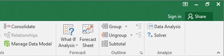
Adding Data Analysis, Solver, or both adds the Analyze group to the Data tab
To add the Data Analysis button to the ribbon
1. In the Backstage view, click Options.
2. In the Excel Options dialog box, click the Add-Ins category.
3. If necessary, click the Manage arrow and then click Excel Add-ins. When Excel Add-ins appears in the Manage box, click Go.
4. In the Add-Ins dialog box, select the Analysis ToolPak check box.
5. Click OK.
To analyze your data by using descriptive statistics
1. On the Data tab, in the Analyze group, click Data Analysis.
2. In the Data Analysis dialog box, click Descriptive Statistics.
3. Click OK.
4. Click in the Input Range box, and then select the cells that contain the data you want to summarize.
5. Select the Summary statistics check box.
6. Click OK.
Skills review
In this chapter, you learned how to:
![]() Examine data by using the Quick Analysis Lens
Examine data by using the Quick Analysis Lens
![]() Define an alternative data set
Define an alternative data set
![]() Define multiple alternative data sets
Define multiple alternative data sets
![]() Analyze data by using data tables
Analyze data by using data tables
![]() Vary your data to get a specific result by using Goal Seek
Vary your data to get a specific result by using Goal Seek
![]() Find optimal solutions by using Solver
Find optimal solutions by using Solver
![]() Analyze data by using descriptive statistics
Analyze data by using descriptive statistics
 Practice tasks
The practice files for these tasks are located in the Excel2016SBS\Ch08 folder. You can save the results of the tasks in the same folder.
Examine data by using the Quick Analysis Lens
Open the PerformQuickAnalysis workbook in Excel, and then perform the following tasks:
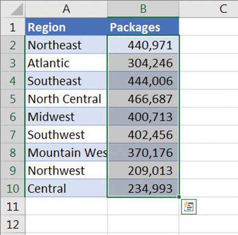
1. Select cells B2:B10.
2. Use the Quick Analysis action button to add a total row to the bottom of the selected range.
3. Use the Quick Analysis action button to add a running total column to the right of the selected range.
Define an alternative data set
Open the CreateScenarios workbook in Excel, and then perform the following tasks:
1. Create a scenario called Overnight that changes the Base Rate value for Overnight and Priority Overnight packages (in cells C6 and C7) to $18.75 and $25.50.
2. Apply the scenario.
3. Undo the scenario application by pressing Ctrl+Z.
4. Close the Scenario Manager dialog box.
Define multiple alternative data sets
Open the ManageMultipleScenarios workbook in Excel, and then perform the following tasks:
1. Create a scenario called HighVolume that increases Ground packages to 17,000,000 and 3Day to 14,000,000.
2. Create a second scenario called NewRates that increases the Ground rate to $9.45 and the 3Day rate to $12.
3. Open the Scenario Manager and create a summary worksheet.
4. Apply the HighVolume scenario, and then apply the NewRates scenario.
5. Close the Scenario Manager dialog box.
Analyze data by using data tables
Open the DefineDataTables workbook in Excel, and then perform the following tasks:
1. On the RateIncreases worksheet, select cells C2:D5.
2. Use the What-If Analysis button to start creating a data table.
3. In the Column input cell box, enter B3.
4. Click OK.
5. On the RateAndVolume worksheet, select cells C2:E6.
6. On the What-If Analysis menu, click Data Table.
7. In the Row input cell box, enter B4.
8. In the Column input cell box, enter B3.
9. Click OK.
Vary your data to get a specific result by using Goal Seek
Open the PerformGoalSeekAnalysis workbook in Excel, and then perform the following tasks:
1. Click cell C4.
2. Open the Goal Seek dialog box.
3. Verify that C4 appears in the Set cell box.
4. In the To value box, enter 20%.
5. In the By changing cell box, enter C3.
6. Click OK.
Find optimal solutions by using Solver
Open the BuildSolverModel workbook in Excel, and then perform the following tasks:
1. Click cell F19, and then open the Solver Parameters dialog box.
2. Verify that cell F19 appears in the Set Objective box, and then select Max.
3. In the By Changing Variable Cells box, select cells C3:E7.
4. Add a constraint to require cell C8 to be less than or equal to the value in cell I10.
5. Add a constraint that requires the values in cells F3:F7 to be less than or equal to the values in cells I3:I7.
6. Make the unconstrained variables non-negative.
7. Solve the model by using the GRG Nonlinear engine.
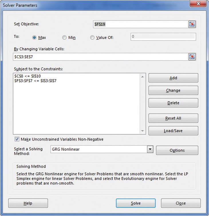
Define your solution by using the Solver Parameters dialog box
8. Click OK to close the Solver Results dialog box and examine the result.
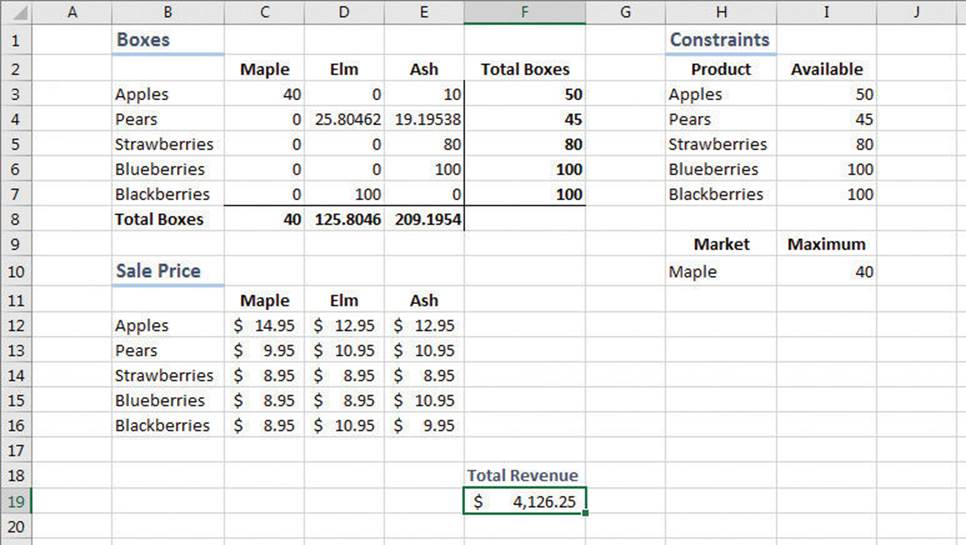
Solver generates a solution without integer constraints
9. Reopen the Solver Parameters dialog box and add another constraint that requires the values in cells C3:E7 to be integers.
10. Click Solve, close the Solver Parameters dialog box, and note how the solution has changed.
Analyze data by using descriptive statistics
Open the UseDescriptiveStatistics workbook in Excel, and then perform the following tasks:
1. Open the Data Analysis dialog box.
2. Click Descriptive Statistics, and then click OK.
3. In the Descriptive Statistics dialog box, click in the Input Range box and select cells C3:C17.
4. Select the Summary statistics check box, and then click OK.
All materials on the site are licensed Creative Commons Attribution-Sharealike 3.0 Unported CC BY-SA 3.0 & GNU Free Documentation License (GFDL)
If you are the copyright holder of any material contained on our site and intend to remove it, please contact our site administrator for approval.
© 2016-2026 All site design rights belong to S.Y.A.