Excel 2016 Formulas (2016)

PART I
Understanding Formula Basics

· Chapter 1: The Excel User Interface in a Nutshell

· Chapter 2: Basic Facts About Formulas

· Chapter 3: Working with Names

Chapter 1
The Excel User Interface in a Nutshell

In This Chapter

· The workings of Excel workbooks

· The Excel user interface

· Protection options

In this chapter, you’ll gain a foundational understanding of the various components in the Excel user interface that you’ll encounter as you move through this book. You’ll get a primer on some of the ways you can protect your formulas and data models before distributing your Excel files.

If you’re already familiar with the basic workings of Excel, you can safely skip to the next chapter. If it has been a while since you’ve worked with Excel, it may be worth your time to scan this chapter to set the stage for the subsequent chapters in the book.

The Workings of Workbooks

When you think about the different components of Excel, it helps to consider a hierarchy of objects. Excel objects include the following:

§ The Excel application itself

§ An Excel workbook

§ A worksheet in a workbook

§ A range in a worksheet

§ A cell in a range

Notice the existence of an object hierarchy: the Excel application contains workbook objects, which contain worksheet objects, which contain range objects, which contain cells. Indeed, Microsoft actually has a name for this inherent hierarchy: the Excel object model.

The core object in the Excel object model is the workbook. Everything that you do in Excel takes place in a workbook.

In Excel 2003 and prior versions, Excel workbook files had the default .xls extension. Excel .xls files are binary files that can be read and manipulated with any version of Excel.

Since the release of Excel 2007, Excel workbooks have been saved as .xlsx files. These .xslsx files are actually compressed folders that can be read and manipulated with Excel 2007 and higher versions.

Inside the compressed folders are a number of files that hold all the information about your workbook, including charts, macros, formatting, and the data in its cells.

Tip

If you’re the curious type, make a copy of an XLSX workbook file and add a .zip extension to the filename. Then unzip the file to see what’s inside.

An Excel workbook can hold any number of sheets. The four types of sheets follow:

§ Worksheets

§ Chart sheets

§ MS Excel 4.0 macro sheets (obsolete, but still supported)

§ MS Excel 5.0 dialog sheets (obsolete, but still supported)

You can open or create as many workbooks as you want (each in its own window), but only one workbook is the active workbook at any given time. Similarly, only one sheet in a workbook is the active sheet. To activate a different sheet, click its corresponding tab at the bottom of the window, or press Ctrl+PgUp (for the previous sheet) or Ctrl+PgDn (for the next sheet). To change a sheet’s name, double-click its Sheet tab and type the new text for the name. Right-clicking a tab brings up a shortcut menu with some additional sheet-manipulation options.

You can also hide the window that contains a workbook by using the View ➜ Window ➜ Hide command. A hidden workbook window remains open but not visible. Use the View ➜ Window ➜ Unhide command to make the window visible again. A single workbook can display in multiple windows (choose View ➜ Window ➜ New Window). Each window can display a different sheet or a different area of the same sheet.

Worksheets

The most common type of sheet is a worksheet, which you normally think of when you think of a spreadsheet. Excel 2016 worksheets have 16,384 columns and 1,048,576 rows.

Note

Versions prior to Excel 2007 support only 256 columns and 65,536 rows. If you open such a file, Excel enters compatibility mode to work with the smaller worksheet grid. To work with the larger grid, you must save the file in one of the newer Excel formats (XLSX or XLSM). Then close the workbook and reopen it. XLSM files can contain macros; XLSX files cannot.

Having access to more cells isn’t the real value of using multiple worksheets in a workbook. Rather, multiple worksheets are valuable because they enable you to organize your work better. Back in the old days, when a spreadsheet file consisted of a single worksheet, developers wasted a lot of time trying to organize the worksheet to hold their information efficiently. Now you can store information on any number of worksheets and still access it instantly.

You have complete control over the column widths and row heights, and you can even hide rows and columns (as well as entire worksheets). You can display the contents of a cell vertically (or at an angle) and even wrap around to occupy multiple lines. In addition, you can merge cells to form a larger cell.

Chart sheets

A chart sheet holds a single chart. Many users ignore chart sheets, preferring to use embedded charts, which are stored on the worksheet’s drawing layer. Using chart sheets is optional, but they make it a bit easier to locate a particular chart, and they prove especially useful for presentations.

Macro sheets and dialog sheets

This section discusses two obsolete Excel features that continue to be supported.

An Excel 4.0 macro sheet, whose purpose is to hold XLM macros, is a worksheet that has some different defaults. XLM is the macro system used in Excel version 4.0 and earlier. This macro system was replaced by VBA in Excel 5.0 and is not discussed in this book.

An Excel 5.0 dialog sheet is a drawing grid that can hold text and controls. In Excel 5.0 and Excel 95, dialog sheets were used to make custom dialog boxes. UserForms were introduced in Excel 97 to replace these sheets.

The Excel User Interface

A user interface (UI) is the means by which an end user communicates with a computer program. The UI for Excel consists of the following components:

§ Tabs and the Ribbon

§ The Quick Access toolbar

§ Right-click (shortcut) menus

§ The mini-toolbar

§ Dialog boxes

§ Keyboard shortcuts

§ Task panes

The Ribbon

The Ribbon is the primary UI component in Excel. The Ribbon provides the user with a single place to conveniently find every commonly used command and dialog box

Note

Before the Ribbon was introduced in Office 2007, almost every Windows program included a more convoluted system of menu bars and toolbars, each of which contained assorted commands and shortcuts.

Tip

A few commands do not appear on the Ribbon but are still available if you know where to look for them. Right-click the Quick Access toolbar and choose Customize Quick Access Toolbar. Excel displays a dialog box with a list of commands that you can add to your Quick Access toolbar. Some of these commands aren’t available elsewhere in the UI. You can also add new commands to the Ribbon; just right-click the Ribbon and select Customize the Ribbon.

Tabs, groups, and tools

The Ribbon is a band of tools that stretches across the top of the Excel window. The Ribbon sports a number of tabs, including Home, Insert, Page Layout, and others. On each tab are groups that contain related tools. On the Home tab, for example, you find the Clipboard group, the Font group, the Alignment group, and others. Within the groups, you’ll find command buttons that activate their respective features.

The Ribbon and all its components resize dynamically as you resize the Excel window horizontally. Smaller Excel windows collapse the tools on compressed tabs and groups, and maximized Excel windows on large monitors show everything that’s available. Even in a small window, all Ribbon commands remain available. You just may need to click a few extra clicks to access them.

Navigation

Using the Ribbon is fairly easy with a mouse or touchscreen. You click a tab and then click a tool. If you prefer to use the keyboard, Microsoft has a feature just for you. Pressing Alt displays tiny squares with shortcut letters in them that hover over their respective tab or tool. Each shortcut letter that you press either executes its command or drills down to another level of shortcut letters. Pressing Esc cancels the letters or moves up to the previous level.

For example, a keystroke sequence of Alt+HBB adds a double border to the bottom of the selection. The Alt key activates the shortcut letters, the H shortcut activates the Home tab, the B shortcut activates the Borders tool menu, and the second B shortcut executes the Bottom Double Border command. Note that you don’t have to keep the Alt key depressed while you press the other keys.

Contextual tabs

The Ribbon contains tabs that are visible only when they are needed. Generally, when a hidden tab appears, it’s because you selected an object or a range with special characteristics (like a chart or a pivot table). A typical example is the Drawing Tools contextual tab. When you select a shape or WordArt object, the Drawing Tools tab is made visible and active. It contains many tools that are applicable only to shapes, such as shape-formatting tools.

Dialog box launchers

At the bottom of many of the Ribbon groups is a small box icon (a dialog box launcher) that opens a dialog box related to that group. Some of the icons open the same dialog boxes but to different areas. For instance, the Font group icon opens the Format Cells dialog box with the Font tab activated. The Alignment group opens the same dialog box but activates the Alignment tab. The Ribbon makes using dialog boxes a far less frequent activity than in the past because most of the commonly used operations can be done directly from the Ribbon.

Galleries and Live Preview

A gallery is a large collection of tools that look like the choice they represent. The Styles gallery, for example, does not just list the name of the style but also displays it in the same formatting that will be applied to the cell.

Although galleries help to give you an idea of what your object will look like when an option is selected, Live Preview takes it to the next level. Live Preview displays your selected object or data as it will look right on the worksheet when you hover over the gallery tool. By hovering over the various tools in the Format Table gallery, you can see exactly what your selected table will look like before you commit to a format.

Backstage View

The File tab is unlike the other tabs. Clicking the File tab doesn’t change the Ribbon but takes you to the Backstage View. This is where you perform most of the document-related activities: creating new workbooks, opening files, saving files, printing, and so on.

The Backstage View also gives you access to the Options dialog button, which opens a dialog box containing dozens of settings for customizing Excel.

Shortcut menus and the mini toolbar

Excel also features dozens of shortcut menus. These menus appear when you right-click after selecting one or more objects. The shortcut menus are context sensitive. In other words, the menu that appears depends on the location of the mouse pointer when you right-click. You can right-click just about anything—a cell, a row or column border, a workbook title bar, and so on.

Right-clicking items often displays the shortcut menu as well as a mini toolbar, which is a floating toolbar that contains a dozen or so of the most popular formatting commands.

Dialog boxes

Some Ribbon commands display a dialog box, from which you can specify options or issue other commands. You’ll find two general classes of dialog boxes in Excel:

§ Modal dialog boxes: When a modal dialog box is displayed, it must be closed to execute the commands. An example is the Format Cells dialog box. None of the options you specify is executed until you click OK. Or click the Cancel button to close the dialog box without making any changes.

§ Modeless dialog boxes: These are stay-on-top dialog boxes. An example is the Find and Replace dialog box. Modeless dialog boxes usually have a Close button rather than OK and Cancel buttons.

Customizing the UI

The Quick Access toolbar is a set of tools that the user can customize. By default, the Quick Access toolbar contains three tools: Save, Undo, and Redo. If you find that you use a particular Ribbon command frequently, right-click the command and choose Add to Quick Access Toolbar. You can make other changes to the Quick Access toolbar from the Quick Access Toolbar tab of the Excel Options dialog box. To access this dialog box, right-click the Quick Access toolbar and choose Customize Quick Access Toolbar.

You can also customize the Ribbon by using the Customize Ribbon tab of the Excel Options dialog box. Choose File ➜ Options to display the Excel Options dialog box.

You can customize the Ribbon in these ways:

§ Add a new tab.

§ Add a new group to a tab.

§ Add commands to a group.

§ Remove groups from a tab.

§ Remove commands from custom groups.

§ Change the order of the tabs.

§ Change the order of the groups within a tab.

§ Change the name of a tab.

§ Change the name of a group.

§ Move a group to a different tab.

§ Reset the Ribbon to remove all customizations.

That’s a fairly comprehensive list of customization options, but there are some actions that you cannot do:

§ You cannot remove built-in tabs, but you can hide them.

§ You cannot remove commands from built-in groups.

§ You cannot change the order of commands in a built-in group.

Task panes

Yet another user interface element is the task pane. Task panes appear automatically in response to several commands. For example, when working with a picture, you can right-click the image and choose Format Picture. Excel responds by displaying the Format Picture task pane. A task pane is similar to a dialog box except that you can keep it visible as long as it’s needed.

By default, the task panes are docked on the right side of the Excel window, but you can move them anywhere you like by clicking the title text and dragging. Excel remembers the last position, so the next time you use a particular task pane, it will be where you left it. There’s no OK button in a task pane. When you’re finished using a task pane, click the Close button (X) in the upper-right corner.

Customizing onscreen display

Excel offers some flexibility regarding onscreen display (status bar, Formula bar, the Ribbon, and so on). For example, click the Ribbon Display Options control (in the title bar), and you can choose how to display the Ribbon. You can hide everything except the title bar, thereby maximizing the amount of visible information.

You can customize the status bar at the bottom of the screen. Right-click the status bar, and you see lots of options that allow you to control what information is displayed.

Many other customizations can be made by choosing File ➜ Options and clicking the Advanced tab. On this tab are several sections that deal with what displays onscreen.

Numeric formatting

Numeric formatting refers to how a value appears in the cell. In addition to choosing from an extensive list of predefined formats, you can create your own custom number formats in the Number tab of the Format Cells dialog box. (Choose the dialog box launcher at the bottom of the Home ➜ Number group.)

Excel applies some numeric formatting automatically, based on the entry. For example, if you precede a value with your local currency symbol (such as a dollar sign), Excel applies Currency number formatting. If you append a percent symbol, Excel applies Percent formatting.

Cross-Ref

Refer to Appendix B, “Using Custom Number Formats,” for additional information about creating custom number formats.

The number format doesn’t affect the actual value stored in the cell. For example, suppose that a cell contains the value 3.14159. If you apply a format to display two decimal places, the number appears as 3.14. When you use the cell in a formula, however, the actual value (3.14159)—not the displayed value—is used.

Stylistic formatting

Stylistic formatting refers to the cosmetic formatting (colors, shading, fonts, borders, and so on) that you apply to make your work look good. The Home ➜ Font and Home ➜ Styles groups contain commands to format your cells and ranges.

Document themes allow you to set many formatting options at once, such as font, colors, and cell styles. The formatting options contained in a theme are designed to work well together. If you’re not feeling particularly artistic, you can apply a theme and know the colors won’t clash. All the commands for themes are in the Themes group of the Page Layout tab.

Don’t overlook Excel’s conditional formatting feature. This handy tool enables you to specify formatting that appears only when certain conditions are met. For example, you can make the cell’s interior red if the cell contains a negative number.

Cross-Ref

See Chapter 19, “Conditional Formatting,” for more information on conditional formatting.

Protection Options

Excel offers a number of different protection options. For example, you can protect formulas from being overwritten or modified, protect a workbook’s structure, and protect your VBA code.

Before distributing any Excel-based work, you should always consider protecting your file using the protection capabilities native to Excel. Although none of Excel’s protection methods are hacker-proof, they do serve to avoid accidental corruption of formulas and to protect sensitive information from unauthorized users.

Securing access to the entire workbook

Perhaps the best way to protect your Excel file is to use Excel’s protection options for file sharing. These options enable you to apply security at the workbook level, requiring a password to view or make changes to the file. This method is by far the easiest to apply and manage because there’s no need to protect each worksheet one at a time. You can apply a blanket protection to guard against unauthorized access and edits. Take a moment to review the file-sharing options, which are as follows:

§ Forcing read-only access to a file until a password is given

§ Requiring a password to open an Excel file

§ Removing workbook-level protection

The next few sections discuss these options in detail.

Permitting read-only access unless a password is given

You can force your workbook to go into read-only mode until the user types the password. This way, you can keep your file safe from unauthorized changes yet still allow authorized users to edit the file.

Here are the steps to force read-only mode:

1. With your file open, click the File tab.

2. To open the Save As dialog box, select Save As and then double-click the This PC icon.

3. In the Save As dialog box, click the Tools button and select General Options (see Figure 1.1). The General Options dialog box appears.

4. Type an appropriate password in the Password to Modify input box (see Figure 1.2), and click OK.

5. Excel asks you to reenter your password, so reenter your chosen password.

6. Save your file to a new name.

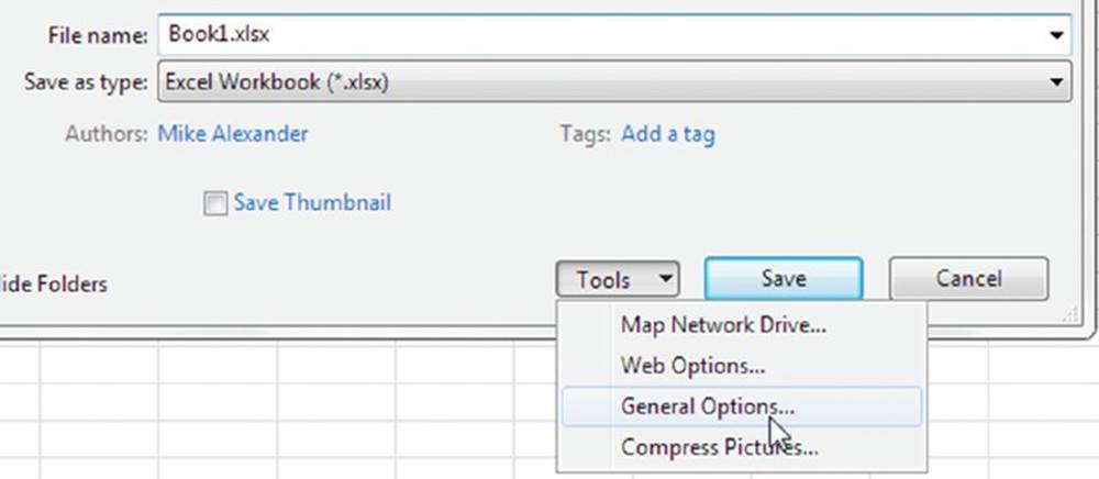
Figure 1.1 The File Sharing options are well hidden away in the Save As dialog box under General Options.

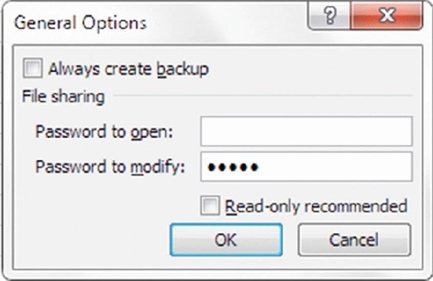
Figure 1.2 Type the password needed to modify the file.

At this point, your file is password protected from unauthorized changes. If you were to open your file, you’d see something similar to Figure 1.3. Failing to type the correct password causes the file to go into read-only mode.

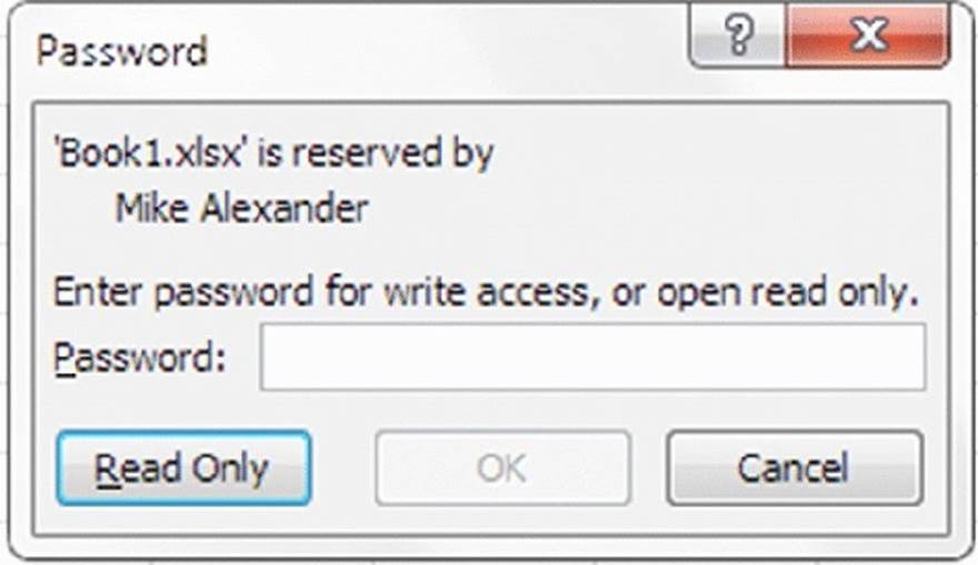
Figure 1.3 A password is now needed to make changes to the file.

Note

Note that Excel passwords are case sensitive, so make sure Caps Lock on your keyboard is in the off position when you’re entering your password.

Requiring a password to open an Excel file

You may have instances in which the data in your Excel files is so sensitive that only certain users are authorized to see it. In these cases, you can require your workbook to receive a password to open it. Here are the steps to set up a password for the file:

1. With your file open, click the File tab.

2. To open the Save As dialog box, select Save As and then double-click the Computer icon.

3. In the Save As dialog box, click the Tools button and select General Options (refer to Figure 1.1). The General Options dialog box opens.

4. Type an appropriate password in the Password to Open text box (as shown in Figure 1.4), and click OK.

5. Excel asks you to reenter your password.

6. Save your file to a new name.

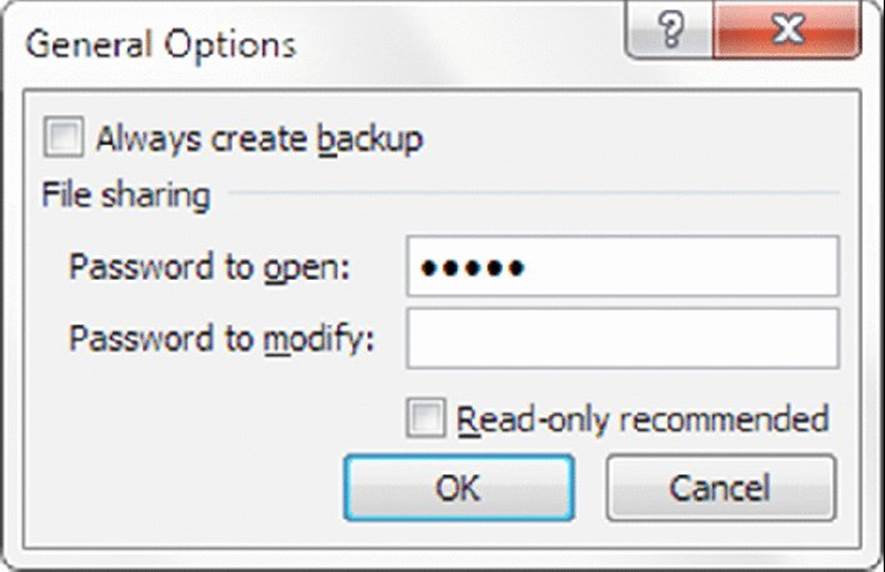
Figure 1.4 Type the password needed to modify the file.

At this point, your file is password protected from unauthorized viewing.

Removing workbook-level protection

Removing workbook-level protection is as easy as clearing the passwords from the General Options dialog box. Here’s how you do it:

1. With your file open, click the File tab.

2. To open the Save As dialog box, select Save As.

3. In the Save As dialog box, click the Tools button and select General Options (refer to Figure 1.1). The General Options dialog box opens.

4. Clear the Password to Open input box as well as the Password to Modify input box, and click OK.

5. Save your file.

Note

When you select the Read-Only Recommended check box in the General Options dialog box (refer to Figure 1.4), you get a message recommending read-only access upon opening the file. This message is only a recommendation and doesn’t prevent anyone from opening the file as read/write.

Limiting access to specific worksheet ranges

You may find that you need to lock specific worksheet ranges, preventing users from taking certain actions. For example, you may not want users to break your formulas inserting or deleting columns and rows. You can prevent this by locking those columns and rows.

Unlocking editable ranges

By default, all cells in a worksheet are set to be locked when you apply worksheet-level protection. You can’t alter the cells on that worksheet in any way. That being said, you may find that you need certain cells or ranges to be editable even in a locked state, as in the example shown in Figure 1.5.

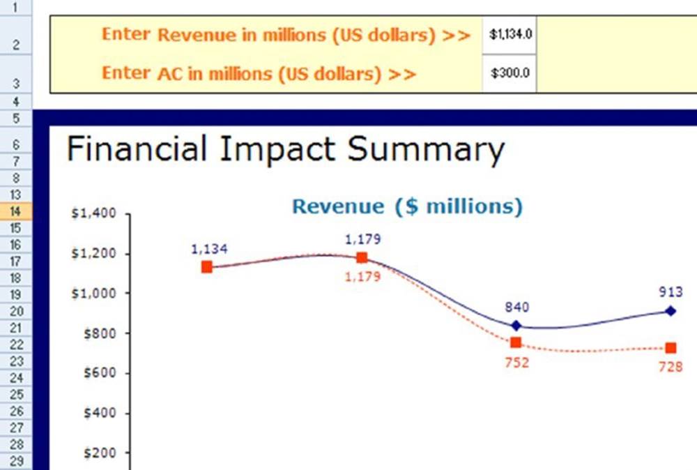
Figure 1.5 Although this sheet is protected, users can enter data into the input cells provided.

Before you protect your worksheet, you can unlock the cell or range of cells that you want users to be able to edit. (The next section shows you how to protect your entire worksheet.) Here’s how to do it:

1. Select the cells you need to unlock.

2. Right-click and select Format Cells.

3. On the Protection tab, as shown in Figure 1.6, deselect the Locked check box.

4. Click OK to apply the change.

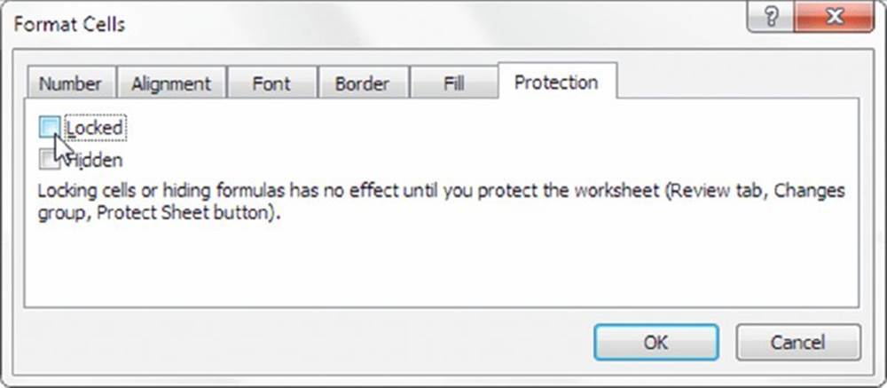
Figure 1.6 To ensure that a cell remains unlocked when the worksheet is protected, deselect the Locked check box.

Applying worksheet protection

After you’ve selectively unlocked the necessary cells, you can begin to apply worksheet protection. Just follow these steps:

1. To open the Protect Sheet dialog box, click the Protect Sheet icon on the Review tab of the Ribbon (see Figure 1.7).

2. Type a password into the text box (see Figure 1.8) and then click OK. This is the password that removes worksheet protection. Note that because you can apply and remove worksheet protection without a password, specifying one is optional.

3. In the list box (see Figure 1.8), select which elements users can change after you protect the worksheet. When a check box is checked for a particular action, Excel prevents users from taking that action.

4. If you provided a password, reenter it.

5. Click OK to apply the worksheet protection.

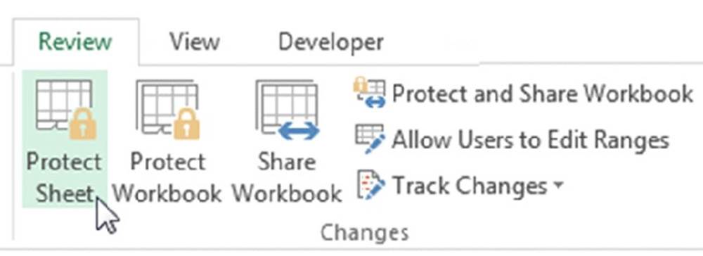
Figure 1.7 Select Protect Sheet in the Review tab.

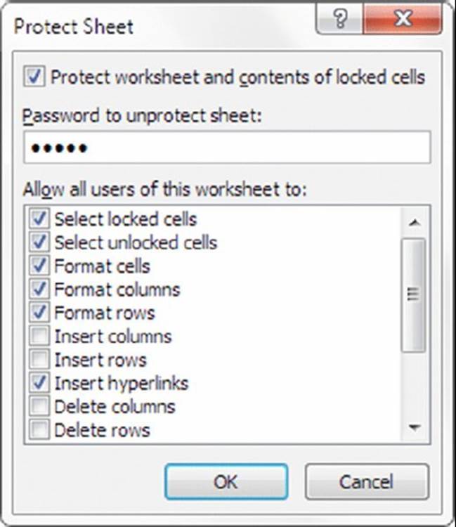
Figure 1.8 Specify a password that removes worksheet protection.

Protecting sheet elements and actions

Take a moment to familiarize yourself with some of the other actions you can limit when protecting a worksheet (refer to Figure 1.8). They are as follows:

§ Select Locked Cells: Allows or prevents the selection of locked cells.

§ Select Unlocked Cells: Allows or prevents the selection of unlocked cells.

§ Format Cells: Allows or prevents the formatting of cells.

§ Format Columns: Allows or prevents the use of column formatting commands, including changing column width or hiding columns.

§ Format Rows: Allows or prevents the use of row formatting commands, including changing row height or hiding rows.

§ Insert Columns: Allows or prevents the inserting of columns.

§ Insert Rows: Allows or prevents the inserting of rows.

§ Insert Hyperlinks: Allows or prevents the inserting of hyperlinks.

§ Delete Columns: Allows or prevents the deleting of columns. Note that if Delete Columns is protected and Insert Columns is not, you can technically insert columns you can’t delete.

§ Delete Rows: Allows or prevents the deleting of rows. Note that if Delete Rows is protected and Insert Rows is not, you can technically insert columns you can’t delete.

§ Sort: Allows or prevents the use of Sort commands. Note that this doesn’t apply to locked ranges. Users can’t sort ranges that contain locked cells on a protected worksheet, regardless of this setting.

§ Use AutoFilter: Allows or prevents use of Excel’s AutoFilter functionality. Users can’t create or remove AutoFiltered ranges on a protected worksheet, regardless of this setting.

§ Use PivotTable Reports: Allows or prevents the modifying, refreshing, or formatting of pivot tables found on the protected sheet.

§ Edit Objects: Allows or prevents the formatting and altering of shapes, charts, text boxes, controls, or other graphics objects.

§ Edit Scenarios: Allows or prevents the viewing of scenarios.

Removing worksheet protection

Just follow these steps to remove any worksheet protection you may have applied:

1. Click the Unprotect Sheet icon on the Review tab.

2. If you specified a password while protecting the worksheet, Excel asks you for that password (see Figure 1.9). Type the password and click OK to immediately remove protection.

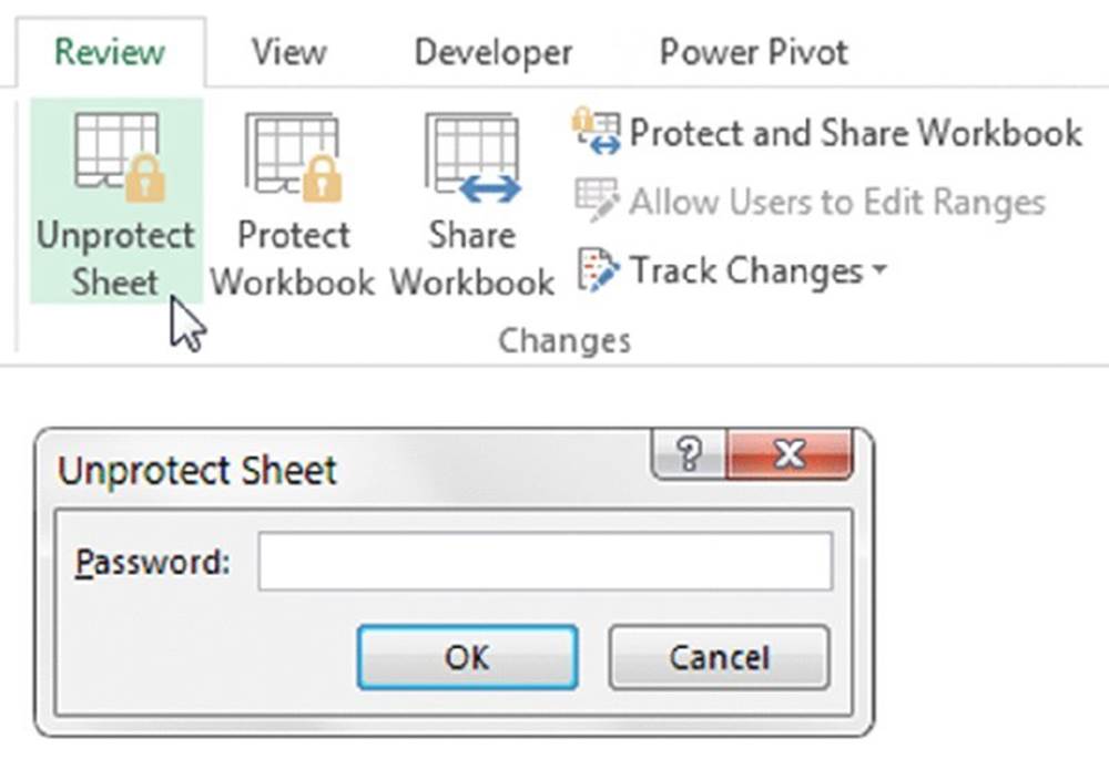
Figure 1.9 The Unprotect Sheet icon removes worksheet protection.

Protecting the workbook structure

If you look under the Review tab in the Ribbon, you see the Protect Workbook icon next to the Protect Sheet icon. Protecting the workbook enables you to prevent users from taking any action that affects the structure of your workbook, such as adding/deleting worksheets, hiding/unhiding worksheets, and naming or moving worksheets. Just follow these steps to protect a workbook:

1. Click the Protect Workbook icon on the Review tab of the Ribbon, which opens the Protect Structure and Windows dialog box as shown in Figure 1.10.

2. Choose which elements you want to protect: workbook structure, windows, or both. When a check box is cleared for a particular action, Excel prevents users from taking that action.

3. If you provided a password, reenter it.

4. Click OK to apply the worksheet protection.

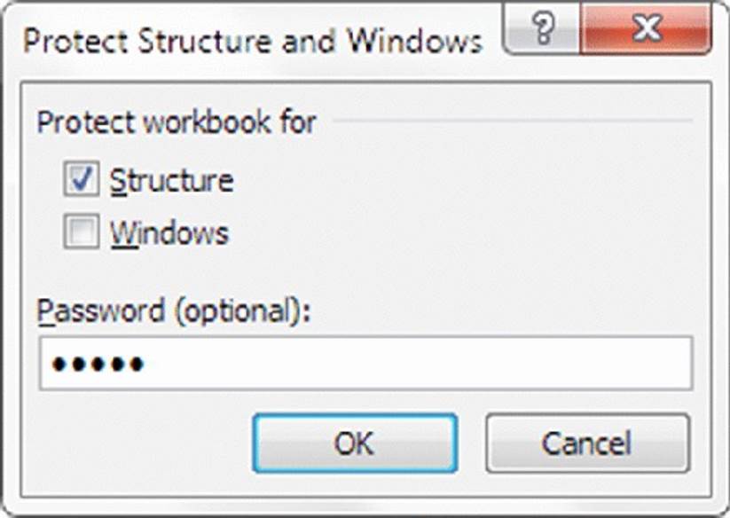
Figure 1.10 The Protect Structure and Windows dialog box.

Selecting Structure prevents users from doing the following:

§ Viewing worksheets that you’ve hidden

§ Moving, deleting, hiding, or changing the names of worksheets

§ Inserting new worksheets or chart sheets

§ Moving or copying worksheets to another workbook

§ Displaying the source data for a cell in a pivot table Values area or displaying pivot table Filter pages on separate worksheets

§ Creating a scenario summary report

§ Using an Analysis ToolPak utility that requires results to be placed on a new worksheet

§ Recording new macros

Choosing Windows prevents users from changing, moving, or sizing the workbook windows while the workbook is opened.