Excel 2016 Formulas (2016)

PART II
Leveraging Excel Functions

Chapter 10
Miscellaneous Calculations

In This Chapter

· Converting between measurement units

· Formulas that demonstrate various ways to round numbers

· Formulas for calculating the various parts of a right triangle

· Calculations for area, surface, circumference, and volume

· Matrix functions to solve simultaneous equations

· Useful formulas for working with normal distributions

This chapter contains reference information that may be useful to you at some point. Consider it a cheat sheet to help you remember the stuff you may have learned but have long since forgotten.

Unit Conversions

You know the distance from New York to London in miles, but your European office needs the numbers in kilometers. What’s the conversion factor?

Excel’s CONVERT function can convert between a variety of measurements in the following categories:

§ Area

§ Distance

§ Energy

§ Force

§ Information

§ Magnetism

§ Power

§ Pressure

§ Speed

§ Temperature

§ Time

§ Volume (or liquid measure)

§ Weight and mass

The CONVERT function requires three arguments: the value that you want to convert, the from-unit, and the to-unit. For example, if cell A1 contains a distance expressed in miles, use this formula to convert miles to kilometers:

=CONVERT(A1,"mi","km")

The second and third arguments are unit abbreviations, which are listed in the Excel Help system. Some of the abbreviations are commonly used, but others aren’t. And, of course, you must use the exact abbreviation. Furthermore, the unit abbreviations are case sensitive, so the following formula returns an error:

=CONVERT(A1,"Mi","km")

The CONVERT function is even more versatile than it seems. When using metric units, you can apply a multiplier. In fact, the first example we presented uses a multiplier. The actual unit abbreviation for the third argument is m for meters. We added the kilo-multipler—k—to express the result in kilometers.

Sometimes you need to use a bit of creativity. For example, if you need to convert 100 km/hour into miles/sec, the formula requires two uses of the CONVERT function:

=CONVERT(100,"km","mi")/CONVERT(1,"hr","sec")

Figure 10.1 shows a conversion table for area measurements. The CONVERT argument codes are in column B and duplicated in row 3. Cell A1 contains a value. The formula in cell C4, which was copied down and across, is

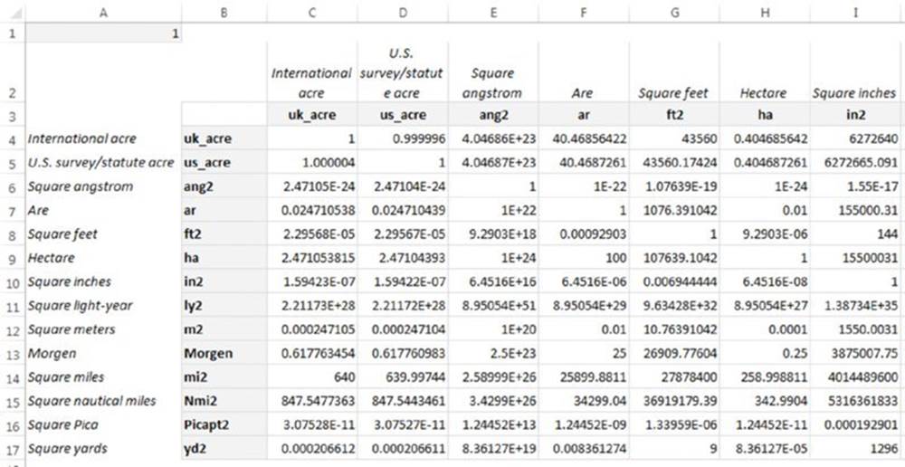
Figure 10.1 A table that lists all the area units supported by the CONVERT function.

=CONVERT($A$1,$B4,C$3)

The table shows, for example, that 1 square foot is equal to 144 square inches. It also shows that one square light year can hold a lot of acres.

By the way, this formula is also a good example of when to use an absolute reference and mixed references in a formula.

On the Web

The workbook shown in Figure 10.1 is available at this book’s website. The filename is area conversion table.xlsx.

Figure 10.2 shows part of a table that lists all the conversion units supported by the CONVERT function. The table can be sorted and filtered and indicates which of the units support the metric prefixes.

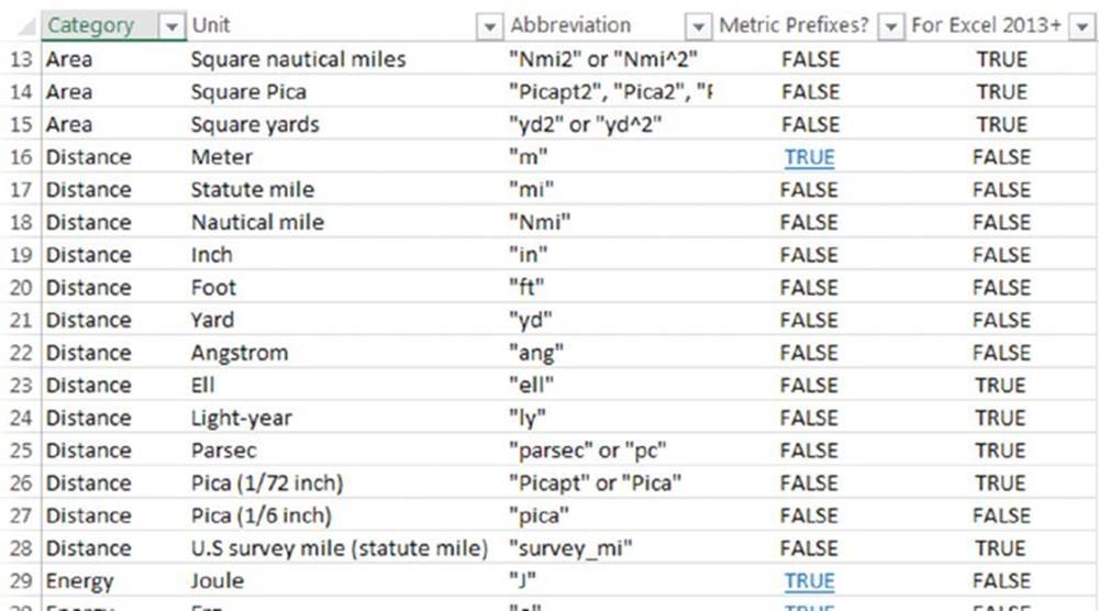
Figure 10.2 A table that lists all the units supported by the CONVERT function.

On the Web

This workbook is available at this book’s website. The filename is conversion units table.xlsx.

If you can’t find a particular unit that works with the CONVERT function, perhaps Excel has another function that will do the job. Table 10.1 lists some other functions that convert between measurement units.

Table 10.1 Other Conversion Functions

* Function available in Excel 2013 and higher versions.

Need to convert other units?

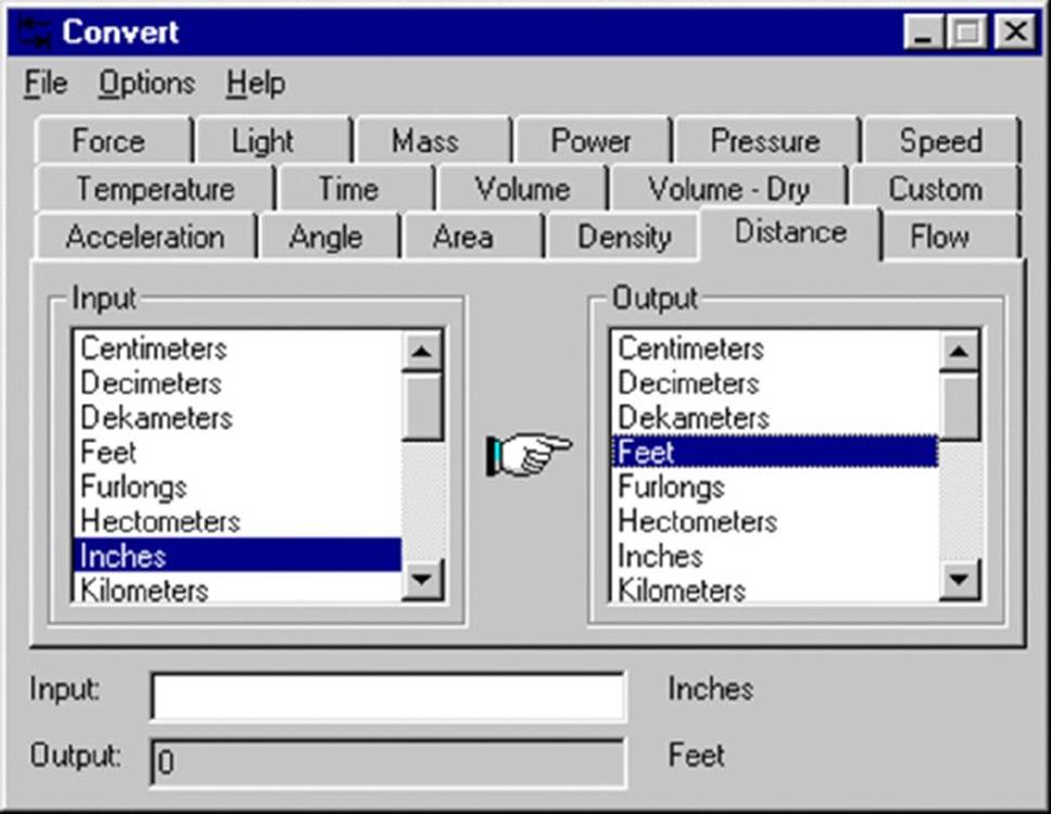
The CONVERT function, of course, doesn’t handle every possible unit conversion. To calculate other unit conversions, you need to find the appropriate conversion factor. The Internet is a good source for such information. Use any web search engine and enter search terms that correspond to the units you use. Likely, you’ll find the information that you need.

Also, you can download a copy of Josh Madison’s popular (and free) Convert software. This excellent program can handle just about any conceivable unit conversion that you throw at it. The URL is http://joshmadison.com/convert-for-windows.

You can use the program to find the conversion factor and then use that value in your formulas.

Rounding Numbers

Excel provides quite a few functions that round values in various ways. Table 10.2 summarizes these functions.

Warning

It’s important to understand the difference between rounding a value and formatting a value. When you format a number to display a specific number of decimal places, formulas that refer to that number use the actual value, which may differ from the displayed value. When you round a number, formulas that refer to that value use the rounded number.

Table 10.2 Excel Rounding Functions

Cross-Ref

Chapter 6, “Working with Dates and Times,” contains examples of rounding time values.

The following sections provide examples of formulas that use various types of rounding.

Basic rounding formulas

The ROUND function is useful for basic rounding to a specified number of digits. You specify the number of digits in the second argument for the ROUND function. For example, the formula that follows returns 123.4. (The value is rounded to one decimal place.)

=ROUND(123.37,1)

If the second argument for the ROUND function is zero, the value is rounded to the nearest integer. The formula that follows, for example, returns 123.00:

=ROUND(123.37,0)

The second argument for the ROUND function can also be negative. In such a case, the number is rounded to the left of the decimal point. The following formula, for example, returns 120.00:

=ROUND(123.37,-1)

The ROUND function rounds either up or down. But how does it handle a number such as 12.5, rounded to no decimal places? You’ll find that the ROUND function rounds such numbers away from zero. The formula that follows, for instance, returns 13.0:

=ROUND(12.5,0)

The next formula returns –13.00. (The rounding occurs away from zero.)

=ROUND(-12.5,0)

To force rounding to occur in a particular direction, use the ROUNDUP or ROUNDDOWN functions. The following formula, for example, returns 12.0. The value rounds down:

=ROUNDDOWN(12.5,0)

The formula that follows returns 13.0. The value rounds up to the nearest whole value:

=ROUNDUP(12.43,0)

Rounding to the nearest multiple

The MROUND function is useful for rounding values to the nearest multiple. For example, you can use this function to round a number to the nearest 5. The following formula returns 135:

=MROUND(133,5)

The second argument for MROUND can be a fractional number. For example, this formula rounds the value in cell A1 to the nearest one-eighth:

=MROUND(A1,1/8)

Rounding currency values

Often, you need to round currency values. For example, you may need to round a dollar amount to the nearest penny. A calculated price may be something like $45.78923. In such a case, you’ll want to round the calculated price to the nearest penny. This may sound simple, but there are actually three ways to round such a value:

§ Round it up to the nearest penny.

§ Round it down to the nearest penny.

§ Round it to the nearest penny. (The rounding may be up or down.)

The following formula assumes that a dollar-and-cents value is in cell A1. The formula rounds the value to the nearest penny. For example, if cell A1 contains $12.421, the formula returns $12.42:

=ROUND(A1,2)

If you need to round the value up to the nearest penny, use the CEILING function. The following formula rounds the value in cell A1 up to the nearest penny. For example, if cell A1 contains $12.421, the formula returns $12.43:

=CEILING(A1,0.01)

To round a dollar value down, use the FLOOR function. The following formula, for example, rounds the dollar value in cell A1 down to the nearest penny. If cell A1 contains $12.421, the formula returns $12.42:

=FLOOR(A1,0.01)

To round a dollar value up to the nearest nickel, use this formula:

=CEILING(A1,0.05)

You’ve probably noticed that many retail prices end in $0.99. If you have an even-dollar price and you want it to end in $0.99, just subtract .01 from the price. Some higher-ticket items are always priced to end with $9.99. To round a price to the nearest $9.99, first round it to the nearest $10.00 and then subtract a penny. If cell A1 contains a price, use a formula like this to convert it to a price that ends in $9.99:

=(ROUND(A1/10,0)*10)-0.01

For example, if cell A1 contains $345.78, the formula returns $349.99.

A simpler approach uses the MROUND function:

=MROUND(A1,10)-0.01

Working with fractional dollars

The DOLLARFR and DOLLARDE functions are useful when working with fractional dollar values, as in stock market quotes.

Consider the value $9.25. You can express the decimal part as a fractional value ($9 1/4, $9 2/8, $9 4/16, and so on). The DOLLARFR function takes two arguments: the dollar amount and the denominator for the fractional part. The following formula, for example, returns 9.1 (and is interpreted as “nine and one-quarter”):

=DOLLARFR(9.25,4)

This formula returns 9.2 (interpreted as “nine and two-eighths”):

=DOLLARFR(9.25,8)

Warning

In most situations, you won’t use the value returned by the DOLLARFR function in other calculations. To perform calculations on such a value, you need to convert it back to a decimal value by using the DOLLARDE function.

The DOLLARDE function converts a dollar value expressed as a fraction to a decimal amount. It also uses a second argument to specify the denominator of the fractional part. The following formula, for example, returns 9.25:

=DOLLARDE(9.1,4)

Working with feet and inches

A problem that has always plagued Excel users is how to work with measurements that are in feet and inches. Excel doesn’t have any special features to make it easy to work with this type of measurement units, but in some cases, you can use the DOLLARDE and DOLLARFR functions.

If you enter 5'9" into a cell, Excel interprets it as a text string—not five feet, nine inches. But if you enter the value as 5.09, you can work with it as a value by using the DOLLARDE function. The following formula returns 5.75, which is the decimal representation of five feet nine inches expressed as fractional feet:

=DOLLARDE(5.09,12)

If you don’t work with fractional inches, you can even create a custom number format. Entering the following custom format will display values as feet and inches.

#" ft". 00" in."

On the Web

This workbook is available at this book’s website. The filename is feet and inches.xlsx.

Using the INT and TRUNC functions

On the surface, the INT and TRUNC functions seem similar. Both convert a value to an integer. The TRUNC function simply removes the fractional part of a number. The INT function rounds a number down to the nearest integer, based on the value of the fractional part of the number.

In practice, INT and TRUNC return different results only when using negative numbers. For example, the following formula returns –14.0:

=TRUNC(-14.2)

The next formula returns –15.0 because –14.3 is rounded down to the next lower integer:

=INT(-14.2)

The TRUNC function takes an additional (optional) argument that’s useful for truncating decimal values. For example, the formula that follows returns 54.33 (the value truncated to two decimal places):

=TRUNC(54.3333333,2)

Rounding to an even or odd integer

The ODD and EVEN functions are provided when you need to round a number up to the nearest odd or even integer. These functions take a single argument and return an integer value. The EVEN function rounds its argument up to the nearest even integer. The ODD function rounds its argument up to the nearest odd integer. Table 10.3 shows some examples of these functions.

Table 10.3 Results Using the EVEN and ODD Functions

Rounding to n significant digits

In some cases, you may need to round a value to a particular number of significant digits. For example, you might want to express the value 1,432,187 in terms of two significant digits: that is, as 1,400,000. The value 9,187,877 expressed in terms of three significant digits is 9,180,000.

If the value is a positive number with no decimal places, the following formula does the job. This formula rounds the number in cell A1 to two significant digits. To round to a different number of significant digits, replace the 2 in this formula with a different number:

=ROUNDDOWN(A1,2-LEN(A1))

For nonintegers and negative numbers, the solution gets a bit trickier. The formula that follows provides a more general solution that rounds the value in cell A1 to the number of significant digits specified in cell A2. This formula works for positive and negative integers and nonintegers:

=ROUND(A1,A2-1-INT(LOG10(ABS(A1))))

For example, if cell A1 contains 1.27845 and cell A2 contains 3, the formula returns 1.28000 (the value, rounded to three significant digits).

Note

Don’t confuse this technique with significant decimal digits, which are the number of digits displayed to the right of the decimal points. It’s an entirely different concept. Also, these formulas make the values less accurate.

Solving Right Triangles

A right triangle has six components: three sides and three angles. Figure 10.3 shows a right triangle with its various parts labeled. Angles are labeled A, B, and C; sides are labeled Hypotenuse, Base, and Height. Angle C is always 90 degrees (or PI/2 radians). If you know any two of these components (excluding Angle C, which is always known), you can use formulas to solve for the others.

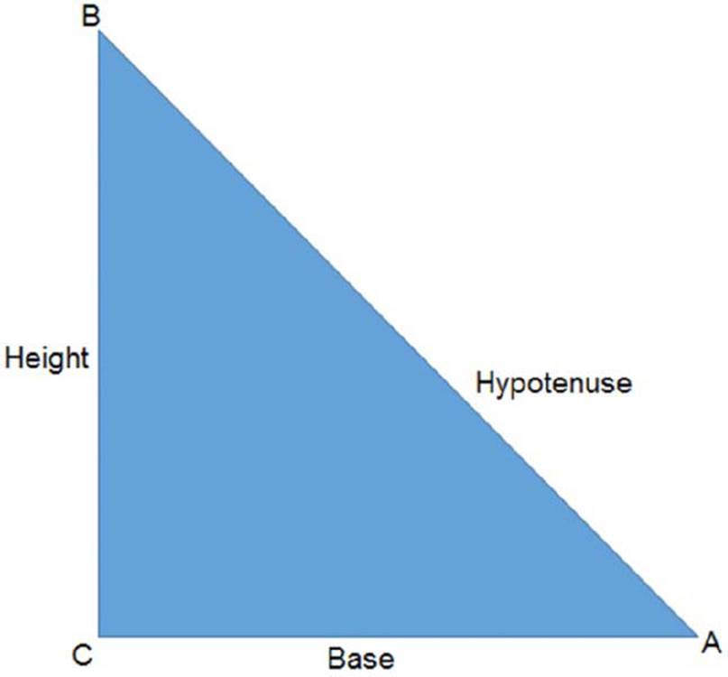
Figure 10.3 A right triangle’s components.

The Pythagorean theorem states that

Height^2 + Base^2 = Hypotenuse^2

Therefore, if you know two sides of a right triangle, you can calculate the remaining side. The formula to calculate a right triangle’s height (given the length of the hypotenuse and base) is as follows:

=SQRT((hypotenuse^2) - (base^2))

The formula to calculate a right triangle’s base (given the length of the hypotenuse and height) is as follows:

=SQRT((hypotenuse^2) - (height^2))

The formula to calculate a right triangle’s hypotenuse (given the length of the base and height) is as follows:

=SQRT((height^2)+(base^2))

Other useful trigonometric identities are

SIN(A) = Height/Hypotenuse

SIN(B) = Base/Hypotenuse

COS(A) = Base/Hypotenuse

COS(B) = Height/Hypotenuse

TAN(A) = Height/Base

SIN(A) = Base/Height

Note

Excel’s trigonometric functions assume that the angle arguments are in radians. To convert degrees to radians, use the RADIANS function. To convert radians to degrees, use the DEGREES function.

If you know the height and base, you can use the following formula to calculate the angle formed by the hypotenuse and base (angle A):

=ATAN(height/base)

The preceding formula returns radians. To convert to degrees, use this formula:

=DEGREES(ATAN(height/base))

If you know the height and base, you can use the following formula to calculate the angle formed by the hypotenuse and height (angle B):

=PI()/2-ATAN(height/base)

The preceding formula returns radians. To convert to degrees, use this formula:

=90-DEGREES(ATAN(height/base))

On the Web

This book’s website contains a workbook —solve right triangle.xlsm— with formulas that calculate various parts of a right triangle, given two known parts. These formulas give you some insight on working with right triangles. The workbook uses a simple VBA macro to enable you to specify the known parts of the triangle.

Figure 10.4 shows a workbook containing formulas to calculate the various parts of a right triangle.

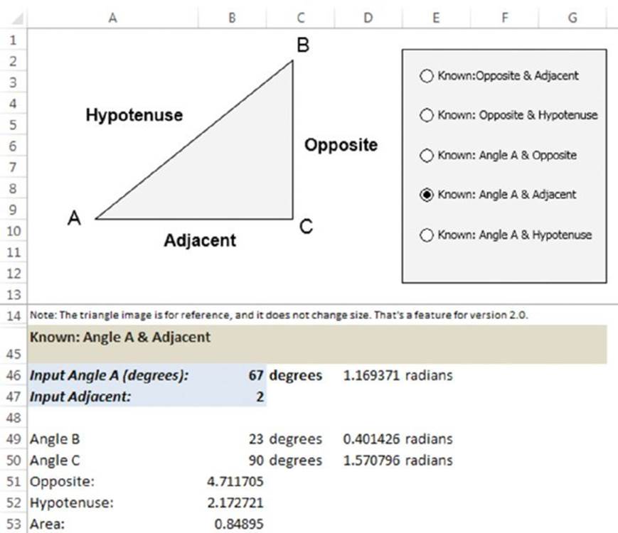
Figure 10.4 This workbook is useful for working with right triangles.

Area, Surface, Circumference, and Volume Calculations

This section contains formulas for calculating the area, surface, circumference, and volume for common two- and three-dimensional shapes.

Calculating the area and perimeter of a square

To calculate the area of a square, square the length of one side. The following formula calculates the area of a square for a cell named side:

=side^2

To calculate the perimeter of a square, multiply one side by 4. The following formula uses a cell named side to calculate the perimeter of a square:

=side*4

Calculating the area and perimeter of a rectangle

To calculate the area of a rectangle, multiply its height by its base. The following formula returns the area of a rectangle, using cells named height and base:

=height*base

To calculate the perimeter of a rectangle, multiply the height by 2 and then add it to the width multiplied by 2. The following formula returns the perimeter of a rectangle, using cells named height and width:

=(height*2)+(width*2)

Calculating the area and perimeter of a circle

To calculate the area of a circle, multiply the square of the radius by (π). The following formula returns the area of a circle. It assumes that a cell named radius contains the circle’s radius:

=PI()*(radius^2)

The radius of a circle is equal to one-half of the diameter.

To calculate the circumference of a circle, multiply the diameter of the circle by (π). The following formula calculates the circumference of a circle using a cell named diameter:

=diameter*PI()

The diameter of a circle is the radius times 2.

Calculating the area of a trapezoid

To calculate the area of a trapezoid, add the two parallel sides, multiply by the height, and then divide by 2. The following formula calculates the area of a trapezoid, using cells named parallel side 1, parallel side 2, and height:

=((parallel side 1+parallel side 2)*height)/2

Calculating the area of a triangle

To calculate the area of a triangle, multiply the base by the height and then divide by 2. The following formula calculates the area of a triangle, using cells named base and height:

=(base*height)/2

Calculating the surface and volume of a sphere

To calculate the surface of a sphere, multiply the square of the radius by (π) and then multiply by 4. The following formula returns the surface of a sphere, the radius of which is in a cell named radius:

=PI()*(radius^2)*4

To calculate the volume of a sphere, multiply the cube of the radius by 4 times (π) and then divide by 3. The following formula calculates the volume of a sphere. The cell named radius contains the sphere’s radius:

=((radius^3)*(4*PI()))/3

Calculating the surface and volume of a cube

To calculate the surface area of a cube, square one side and multiply by 6. The following formula calculates the surface of a cube using a cell named side, which contains the length of a side of the cube:

=(side^2)*6

To calculate the volume of a cube, raise the length of one side to the third power. The following formula returns the volume of a cube, using a cell named side:

=side^3

Calculating the surface and volume of a rectangular solid

The following formula calculates the surface of a rectangular solid using cells named height, width, and length:

=(length*height*2)+(length*width*2)+(width*height*2)

To calculate the volume of a rectangular solid, multiply the height by the width by the length:

=height*width*length

Calculating the surface and volume of a cone

The following formula calculates the surface of a cone (including the surface of the base). This formula uses cells named radius and height:

=PI()*radius*(SQRT(height^2+radius^2)+radius)

To calculate the volume of a cone, multiply the square of the radius of the base by (π), multiply by the height, and then divide by 3. The following formula returns the volume of a cone, using cells named radius and height:

=(PI()*(radius^2)*height)/3

Calculating the volume of a cylinder

To calculate the volume of a cylinder, multiply the square of the radius of the base by (π) and then multiply by the height. The following formula calculates the volume of a cylinder, using cells named radius and height:

=(PI()*(radius^2)*height)

Calculating the volume of a pyramid

Calculate the area of the base, multiply by the height, and then divide by 3. This formula calculates the volume of a pyramid. It assumes cells named width (the width of the base), length (the length of the base), and height (the height of the pyramid).

=(width*length*height)/3

Solving Simultaneous Equations

This section describes how to use formulas to solve simultaneous linear equations. The following is an example of a set of simultaneous linear equations:

3x + 4y = 8

4x + 8y = 1

Solving a set of simultaneous equations involves finding the values for x and y that satisfy both equations. For this set of equations, the solution is as follows:

x = 7.5

y = –3.625

The number of variables in the set of equations must be equal to the number of equations. The preceding example uses two equations with two variables. Three equations are required to solve for three variables (x, y, and z).

The general steps for solving a set of simultaneous equations follow. See Figure 10.5, which uses the equations presented at the beginning of this section.

1. Express the equations in standard form. If necessary, use simple algebra to rewrite the equations such that all the variables appear on the left side of the equal sign. The two equations that follow are identical, but the second one is in standard form:

2. 3x –8 = –4y

3x + 4y = 8

2. Place the coefficients in an n × n range of cells, where n represents the number of equations. In Figure 10.5, the coefficients are in the range I2:J3.

3. Place the constants (the numbers on the right side of the equal sign) in a vertical range of cells. In Figure 10.5, the constants are in the range L2:L3.

4. Use an array formula to calculate the inverse of the coefficient matrix. In Figure 10.5, the following array formula is entered into the range I6:J7. (Remember to press Ctrl+Shift+Enter to enter an array formula, and omit the curly brackets.)

{=MINVERSE(I2:J3)}

5. Use an array formula to multiply the inverse of the coefficient matrix by the constant matrix. In Figure 10.5, the following array formula is entered into the range J10:J11. This range holds the solution:

{=MMULT(I6:J7,L2:L3)}

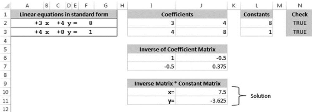
Figure 10.5 Using formulas to solve simultaneous equations.

Cross-Ref

See Chapter 14, “Introducing Arrays,” for more information on array formulas.

On the Web

You can access the workbook, simultaneous equations.xlsx, shown in Figure 10.5, from this book’s website. This workbook solves simultaneous equations with two or three variables.

Working with Normal Distributions

In statistics, a common topic is the normal distribution, also known as a bell curve. Excel has several functions designed to work with normal distributions. This is not a statistics book, so we assume that if you’re reading this section, you’re familiar with the concept.

On the Web

The examples in this section are available at this book’s website. The filename is normal distribution.xlsx.

Figure 10.6 shows a workbook containing formulas that generate the two charts: a normal distribution and a cumulative normal distribution.

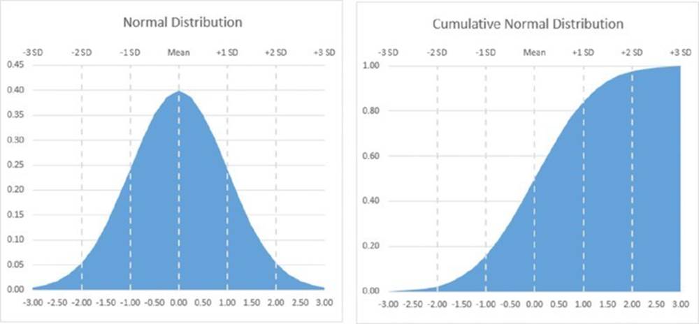
Figure 10.6 Using formulas to calculate a normal distribution and a cumulative normal distribution.

The formulas use the values entered into cell B1 (name Mean) and cell B2 (named SD, for standard deviation). The values calculated cover the mean plus/minus three standard deviations. Column A contains formulas that generate 25 equally spaced intervals, ranging from –3 standard deviations to +3 standard deviations.

A normal distribution with a mean of 0 and a standard deviation of 1 is known as the “standard normal distribution.” The worksheet is set up to work with any mean and any standard deviation.

Formulas in column B calculate the height of the normal curve for each of the 25 values in column A. Cell B5 contains this formula, which is copied down the column:

=NORM.DIST(A5,Mean,SD,FALSE)

The formula in cell C5 is the same, except for the last argument. When that argument is TRUE, the function returns the cumulative probability:

=NORMDIST(A5,Mean,SD,TRUE)

Figure 10.7 shows a worksheet with 2,600 data points in column A (named Data) that is approximately normally distributed. Formulas in column D calculate some basic statistics for this data: N (the number of data points), the minimum, the maximum, the mean, and the standard deviation.

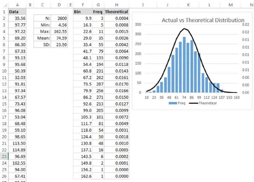
Figure 10.7 Comparing a set of data with a normal distribution.

Column F contains an array formula that creates 25 equal-interval bins that cover the complete range of the data. It uses the technique described in Chapter 7, “Counting and Summing Techniques.” The multicell array formula, entered in F2:F26 (named Bins), is

=MIN(Data)+(ROW(INDIRECT("1:25"))*(MAX(Data)-MIN(Data)+1)/25)-1

Column G also contains a multicell array formula that calculates the frequency for each of the 25 bins:

=FREQUENCY(Data,Bins)

The data in column G is displayed in the chart as columns and uses the axis on the left.

Column H contains formulas that calculate the value of the theoretical normal distribution, using the mean and standard deviation of the Data range.

The formula in cell H2, which is copied down the column, is

=NORMDIST(F2,$D$5,$D$6,FALSE)

In the chart, the values in column H are plotted as a line and use the right axis. As you can see, the data conforms fairly well to the normal distribution. There are goodness-of-fit tests to determine the “normality” of a set of data samples, but that’s beyond the scope of this book.