Excel 2016 Formulas (2016)

PART III
Financial Formulas

· Chapter 11: Borrowing and Investing Formulas

· Chapter 12: Discounting and Depreciation Formulas

· Chapter 13: Financial Schedules

Chapter 11
Borrowing and Investing Formulas

In This Chapter

· A brief overview of the Excel functions that deal with the time value of money

· Formulas that perform various types of loan calculations

· Formulas that perform various types of investment calculations

It’s a safe bet that the most common use for Excel is to perform calculations involving money. Every day, people make hundreds of thousands of financial decisions based on the numbers that are calculated in a spreadsheet. These decisions range from simple (Can I afford to buy a new car?) to complex (Will purchasing XYZ Corporation result in a positive cash flow in the next 18 months?). This is the first of three chapters that discuss financial calculations you can perform with the assistance of Excel.

The Time Value of Money

The face value of money may not always be what it seems. A key consideration is the time value of money. This concept involves calculating the value of money in the past, present, or future. It’s based on the premise that money increases in value over time because of interest earned by the money. In other words, a dollar invested today will be worth more tomorrow.

For example, imagine that your rich uncle decided to give away some money and asked you to choose one of the following options:

§ Receive $8,000 today

§ Receive $9,500 in one year

§ Receive $12,000 in five years

§ Receive $150 per month for five years

If your goal is to maximize the amount received, you need to take into account not only the face value of the money but also the time value of the money when it arrives in your hands.

The time value of money depends on your perspective. In other words, you’re either a lender or a borrower. When you take out a loan to purchase an automobile, you’re a borrower, and the institution that provides the funds to you is the lender. When you invest money in a bank savings account, you’re a lender; you’re lending your money to the bank, and the bank is borrowing it from you.

Several concepts contribute to the time value of money:

§ Present value (PV): This is the principal amount. If you deposit $5,000 in a bank savings account, this amount represents the principal, or present value, of the money you invested. If you borrow $15,000 to purchase a car, this amount represents the principal, or present value, of the loan. The present value may be positive or negative.

§ Future value (FV): This is the principal plus interest. If you invest $5,000 for five years and earn 3% annual interest, your investment is worth $5,796.37 at the end of the five-year term. This amount is the future value of your $5,000 investment. If you take out a three-year car loan for $15,000 and make monthly payments based on a 5.25% annual interest rate, you pay a total of $16,244.97. This amount represents the principal plus the interest you paid. The future value may be positive or negative, depending on the perspective (lender or borrower).

§ Payment (PMT): This is either principal or principal plus interest. If you deposit $100 per month into a savings account, $100 is the payment. If you have a monthly mortgage payment of $1,025, this amount is made up of principal and interest.

§ Interest rate: Interest is a percentage of the principal, usually expressed on an annual basis. For example, you may earn 2.5% annual interest on a bank CD (certificate of deposit). Or your mortgage loan may have a 6.75% interest rate.

§ Period: This represents the point in time when interest is paid or earned, such as a bank CD that pays interest quarterly or an auto loan that requires monthly payments.

§ Term: This is the amount of time of interest. A 12-month bank CD has a term of one year. A 30-year mortgage loan has a term of 360 months.

Loan Calculations

This section describes how to calculate various components of a loan. Think of a loan as consisting of the following components:

§ The loan amount

§ The interest rate

§ The number of payment periods

§ The periodic payment amount

If you know any three of these components, you can create a formula to calculate the unknown component.

Note

All the loan calculations in this section assume a fixed-rate loan with a fixed term.

Worksheet functions for calculating loan information

This section describes six commonly used financial functions: PMT, PPMT, IPMT, RATE, NPER, and PV. For information about the arguments used in these functions, see Table 11.1. In the sections that follow, you’ll notice that many of the functions also serve as arguments of other functions. This is quite logical, as all of these terms are interconnected with each other in a variety of ways.

Table 11.1 Financial Function Arguments

PMT

The PMT function answers the question, “How much will my payment be for a loan with constant payment amounts and a fixed interest rate?” The syntax for the PMT function follows:

PMT(rate,nper,pv,fv,type)

The following formula returns the monthly payment amount for a $5,000 loan with a 6% annual percentage rate. The loan has a term of four years (48 months).

=PMT(6&/12,48,5000)

This formula returns ($117.43), the monthly payment for the loan. The first argument, rate, is the annual rate divided by the number of months in a year to convert it to monthly rate. Also, notice that the third argument (pv, for present value) is positive because it’s a cash inflow to you (the borrower), and the result is negative because the payments are cash outflows.

PPMT

The PPMT function answers the question, “How much of a particular payment is applied to the principal?” The syntax for the PPMT function follows:

PPMT(rate,per,nper,pv,fv,type)

The following formula returns the amount paid to principal for the first month of a $5,000 loan with a 6% annual percentage rate. The loan has a term of four years (48 months):

=PPMT(6&/12,1,48,5000)

The formula returns ($92.43) for the principal, which is about 78.7% of the total loan payment. If we change the second argument to 48 (to calculate the principal amount for the last payment), the formula returns ($116.84), or about 99.5% of the total loan payment.

Note

To calculate the cumulative principal paid between any two payment periods, use the CUMPRINC function. This function uses two additional arguments: start_period and end_period. In Excel versions prior to Excel 2007, CUMPRINC is available only when you install the Analysis ToolPak add-in.

IPMT

The IPMT function answers the question, “How much of a particular payment is for interest?” Here’s the syntax for the IPMT function:

IPMT(rate,per,nper,pv,fv,type)

The following formula returns the amount paid to interest for the first month of a $5,000 loan with a 6% annual percentage rate. The loan has a term of four years (48 months):

=IPMT(6&/12,1,48,5000)

This formula returns an interest amount of $25.00. By the last payment period for the loan, the interest payment is only $0.58. If you add the result of IPMT to PPMT for the same payment, you get the result of PMT (the total payment amount).

Note

To calculate the cumulative interest paid between any two payment periods, use the CUMIPMT function. This function uses two additional arguments: start_period and end_period. In Excel versions prior to Excel 2007, CUMIPMT is available only when you install the Analysis ToolPak add-in.

RATE

The RATE function answers the question, “What is the interest rate of my loan given the number of payment periods, the payment amount, and the loan amount?” Here’s the syntax for the RATE function:

RATE(nper,pmt,pv,fv,type,guess)

The following formula calculates the annual interest rate for a 48-month loan for $5,000 that has a monthly payment amount of $117.43:

=RATE(48,-117.43,5000)*12

This formula returns 6.00%. Notice that the result of the function is multiplied by 12 to get the annual percentage rate.

NPER

The NPER function answers the question, “How many payments are needed to pay off my loan given the loan amount, interest rate, and periodic payment amount?” Here’s the syntax for the NPER function:

NPER(rate,pmt,pv,fv,type)

The following formula calculates the number of payment periods for a $5,000 loan that has a monthly payment amount of $117.43. The loan has a 6% annual interest rate:

=NPER(6&/12,-117.43,5000)

This formula returns 47.997 (that is, 48 months). The monthly payment was rounded to the nearest penny, causing the minor discrepancy.

PV

The PV function answers the question, “How much can I borrow given the interest rate, the number of periods, and the payment amount?” The syntax for the PV function follows:

PV(rate,nper,pmt,fv,type)

The next formula calculates the amount of a loan that can be paid off with 48 monthly payments of $117.43 at an annual interest rate of 6%:

=PV(6&/12,48,-117.43)

This formula returns $5,000.21. The monthly payment was rounded to the nearest penny, causing the $0.21 discrepancy.

A loan calculation example

Figure 11.1 shows a worksheet set up to calculate the periodic payment amount for a loan.

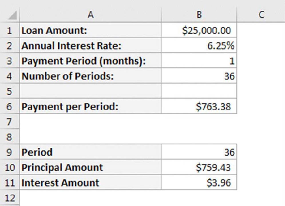
Figure 11.1 Using the PMT function to calculate a periodic loan payment amount.

On the Web

The workbook described in this section is available at this book’s website. The file is named loan payment.xlsx.

The loan amount is in cell B1, and the annual interest rate is in cell B2. Cell B3 contains the payment period expressed in months. For example, if cell B3 is 1, the payment is due monthly. If cell B3 is 3, the payment is due every three months, or quarterly. Cell B4 contains the number of periods of the loan. The example shown in this figure calculates the payment for a $25,000 loan at 6.25% annual interest with monthly payments for 36 months. The formula in cell B6 follows:

=PMT(B2*(B3/12),B4,-B1)

Notice that the first argument is an expression that calculates the periodic interest rate by using the annual interest rate and the payment period. Therefore, if payments are made quarterly on a three-year loan, the payment period is 3, the number of periods is 12, and the periodic interest rate is calculated as the annual interest rate multiplied by three-twelfths.

The worksheet in Figure 11.1 is set up to calculate the principal and interest amount for a particular payment period. Cell B9 contains the payment period used by the formulas in B10:B11. (The payment period must be less than or equal to the value in cell B4.)

The formula in cell B10, shown here, calculates the amount of the payment that goes toward principal for the payment period in cell B9:

=PPMT(B2*(B3/12),B9,B4,-B1)

The following formula, in cell B11, calculates the amount of the payment that goes toward interest for the payment period in cell B9:

=IPMT(B2*(B3/12),B9,B4,-B1)

The sum of B10 and B11 is equal to the total loan payment calculated in cell B6. However, the relative proportion of principal and interest amounts varies with the payment period. (An increasingly larger proportion of the payment is applied toward principal as the loan progresses.) Figure 11.2 shows the principal and interest portions graphically.

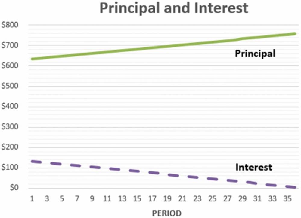
Figure 11.2 This chart shows how the interest and principal amounts vary during the payment periods of a loan.

Credit card payments

Do you ever wonder how long it takes to pay off a credit card balance if you make the minimum payment amount each month? Figure 11.3 shows a worksheet set up to make this type of calculation.

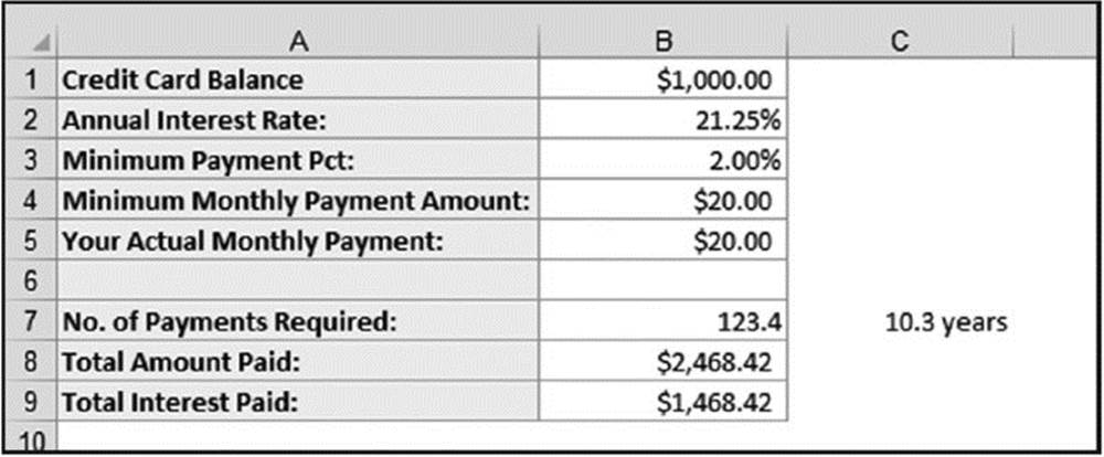
Figure 11.3 This worksheet calculates the number of payments required to pay off a credit card balance by paying the minimum payment amount each month.

On the Web

The workbook shown in Figure 11.3 is available at this book’s website. The file is named credit card payments.xlsx.

Range B1:B5 stores input values. In this example, the credit card has a balance of $1,000, and the lender charges a 21.25% annual percentage rate (APR). The minimum payment is 2.00% (typical of many credit card lenders). Therefore, the minimum payment amount for this example is $20. You can enter a different payment amount in cell B5, but it must be large enough to pay off the loan. For example, you may choose to pay $50 per month to pay off the balance more quickly. However, paying $10 per month isn’t sufficient, and the formulas return an error.

Range B7:B9 holds formulas that perform various calculations. The formula in cell B7, which follows, calculates the number of months required to pay off the balance:

=NPER(B2/12,B5,-B1,0)

The formula in B8 calculates the total amount you will pay. This formula follows:

=B7*B5

The formula in cell B9 calculates the total interest paid:

=B8-B1

In this example, it would take about 123 months (more than 10 years) to pay off the credit card balance if the borrower made only the minimum monthly payment. The total interest paid on the $1,000 loan would be $1,468.42. This calculation assumes, of course, that no additional charges are made on the account. This example may help explain why you receive so many credit card solicitations in the mail.

Figure 11.4 shows some additional calculations for the credit card example. For example, if you want to pay off the credit card in 12 months, you need to make monthly payments of $93.23. (This amount results in total payments of $1,118.81 with total interest of $118.81.) The formula in B13 follows:

=PMT($B$2/12,A13,-$B$1)

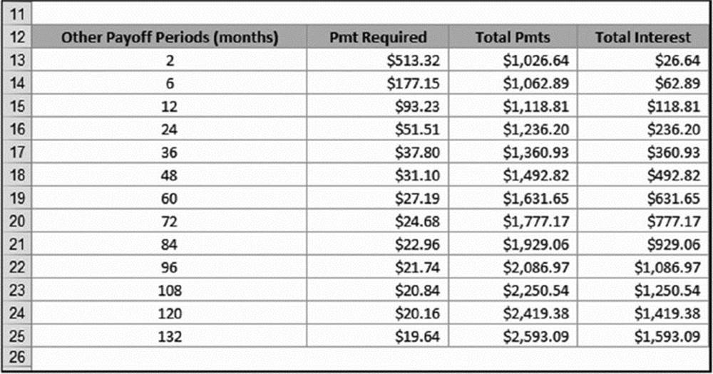
Figure 11.4 The second column shows the payment required to pay off the credit card balance for various payoff periods.

Creating a loan amortization schedule

A loan amortization schedule is a table of values that shows various types of information for each payment period of a loan. Figure 11.5 shows a worksheet that uses formulas to calculate an amortization schedule.

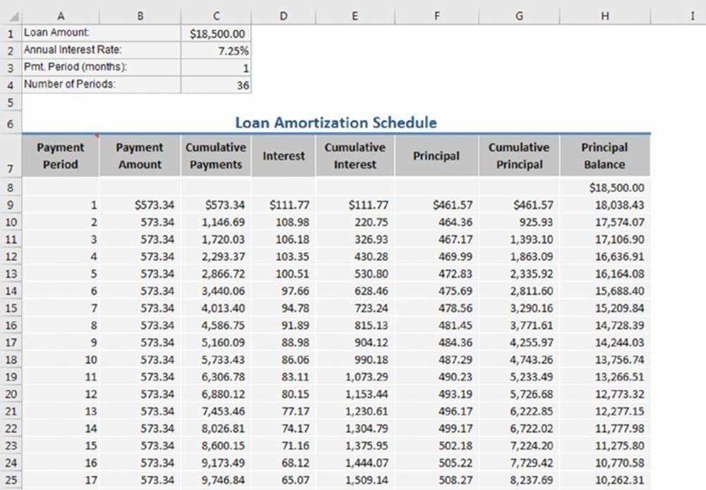
Figure 11.5 A loan amortization schedule.

On the Web

This workbook is available on this book’s website. The file is named loan amortization schedule.xlsx.

The loan parameters are entered into C1:C4, and the formulas beginning in row 9 use these values for the calculations. Table 11.2 shows the formulas in row 9 of the schedule. These formulas were copied down to row 488. Therefore, the worksheet can calculate amortization schedules for a loan with as many as 480 payment periods (40 years of monthly payments).

Table 11.2 Formulas Used to Calculate an Amortization Schedule

Note

Formulas in the rows that extend beyond the number of payments return an error value. The worksheet uses conditional formatting to hide the data in these rows.

Cross-Ref

See Chapter 19, “Conditional Formatting,” for more information about conditional formatting.

Calculating a loan with irregular payments

So far, the loan calculation examples in this chapter have involved loans with regular periodic payments. In some cases, loan payback is irregular. For example, you may loan some money to a friend without a formal agreement as to how he’ll pay the money back. You still collect interest on the loan, so you need a way to perform the calculations based on the actual payment dates.

Figure 11.6 shows a worksheet set up to keep track of such a loan. The annual interest rate for the loan is stored in cell B1 (named APR). The original loan amount and loan date are stored in row 5. Notice that the loan amount is entered as a negative value in cell B5. Formulas, beginning in row 6, track the irregular loan payments and perform calculations.

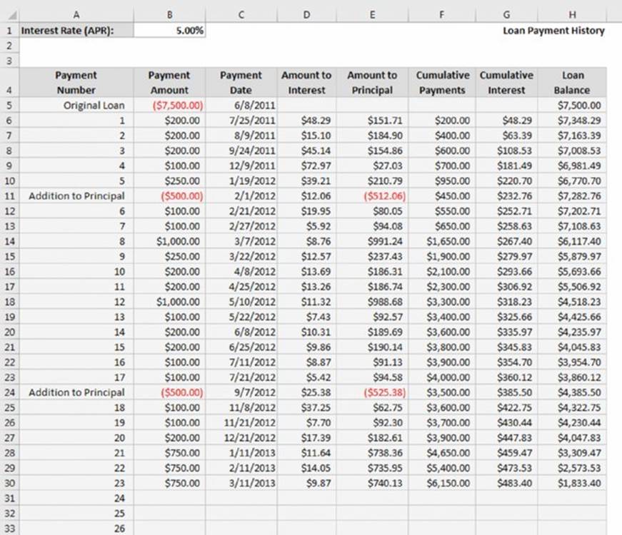
Figure 11.6 This worksheet tracks loan payments that are made on an irregular basis.

Column B stores the payment amount made on the date in column C. Notice that the payments are not made on a regular basis. Also, notice that in two cases (row 11 and row 24), the payment amount is negative. These entries represent additional borrowed money added to the loan balance. Formulas in columns D and E calculate the amount of the payment credited toward interest and principal. Columns F and G keep a running tally of the cumulative payments and interest amounts. Formulas in column H compute the new loan balance after each payment.

Table 11.3 lists and describes the formulas in row 6. Note that each formula uses an IF function to determine whether the payment date in column C is missing. If so, the formula returns an empty string, so no data appears in the cell.

Table 11.3 Formulas to Calculate a Loan with Irregular Payments

Note that the formula in cell D6 assumes that the year has 365 days. A more precise formula uses the YEARFRAC function, which calculates the fraction of a year when a leap year is involved:

=IF(C6<>"",YEARFRAC(C6,C5,1)*H5*APR,"")

On the Web

This workbook is available at this book’s website. The filename is irregular payments.xlsx.

Investment Calculations

Investment calculations involve calculating interest on fixed-rate investments, such as bank savings accounts, CDs, and annuities. You can make these interest calculations for investments that consist of a single deposit or multiple deposits.

On the Web

This book’s website contains a workbook with all the interest calculation examples in this section. The file is named investment calculations.xlsx.

Future value of a single deposit

Many investments consist of a single deposit that earns interest over the term of the investment. This section describes calculations for simple interest and compound interest.

Calculating simple interest

Simple interest refers to the fact that interest payments are not compounded. The basic formula for computing interest is this:

Interest=Principal*Rate*Term

For example, suppose that you deposit $1,000 into a bank CD that pays a 3% simple annual interest rate. After one year, the CD matures, and you withdraw your money. The bank adds $30, and you walk away with $1,030. In this case, the interest earned is calculated by multiplying the principal ($1,000) by the interest rate (0.03) by the term (one year).

If the investment term is less than one year, the simple interest rate is adjusted accordingly, based on the term. For example, $1,000 invested in a six-month CD that pays 3% simple annual interest earns $15.00 when the CD matures. In this case, the annual interest rate multiplies by six-twelfths.

Figure 11.7 shows a worksheet set up to make simple interest calculations. The formula in cell B7, shown here, calculates the interest due at the end of the term:

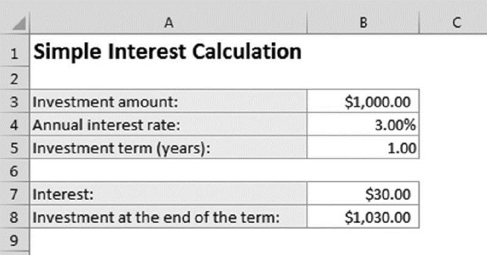
Figure 11.7 This worksheet calculates simple interest payments.

=B3*B4*B5

The formula in B8 simply adds the interest to the original investment amount.

Calculating compound interest

Most fixed-term investments pay interest by using some type of compound interest calculation. Compound interest refers to interest credited to the investment balance, and the investment then earns interest on the interest.

For example, suppose that you deposit $1,000 into a bank CD that pays 3% annual interest rate, compounded monthly. Each month, the interest is calculated on the balance, and that amount is credited to your account. The next month’s interest calculation is based on a higher amount because it also includes the previous month’s interest payment. One way to calculate the final investment amount involves a series of formulas (see Figure 11.8).

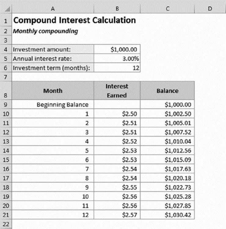
Figure 11.8 Using a series of formulas to calculate compound interest.

Column B contains formulas to calculate the interest for one month. For example, the formula in B10 is

=C9*($B$5*(1/12))

The formulas in column C simply add the monthly interest amount to the balance. For example, the formula in C10 is

=C9+B10

At the end of the 12-month term, the CD balance is $1,030.42. In other words, monthly compounding results in an additional $0.42 (compared with simple interest).

You can use the FV (future value) function to calculate the final investment amount without using a series of formulas. Figure 11.9 shows a worksheet set up to calculate compound interest. Cell B6 is an input cell that holds the number of compounding periods per year. For monthly compounding, the value in B6 would be 12. For quarterly compounding, the value would be 4. For daily compounding, the value would be 365. Cell B7 holds the term of the investment expressed in years.

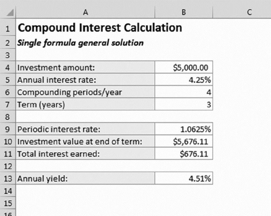
Figure 11.9 Using a single formula to calculate compound interest.

Cell B9 contains the following formula that calculates the periodic interest rate. This value is the interest rate used for each compounding period:

=B5*(1/B6)

The formula in cell B10 uses the FV function to calculate the value of the investment at the end of the term. The formula follows:

=FV(B9,B6*B7,,-B4)

The first argument for the FV function is the periodic interest rate, which is calculated in cell B9. The second argument represents the total number of compounding periods. The third argument (pmt) is omitted, and the fourth argument is the original investment amount (expressed as a negative value).

The total interest is calculated with a simple formula in cell B11:

=B10-B4

Another formula, in cell B13, calculates the annual yield on the investment:

=(B11/B4)/B7

For example, suppose that you deposit $5,000 into a three-year CD with a 4.25% annual interest rate compounded quarterly. In this case, the investment has four compounding periods per year, so you enter 4 into cell B6. The term is three years, so you enter 3 into cell B7. The formula in B10 returns $5,676.11.

Perhaps you want to see how this rate stacks up against another account that offers daily compounding. Figure 11.10 shows a calculation with daily compounding using a $5,000 investment (compare this with Figure 11.9). As you can see, the difference is small ($679.88 versus $676.11). Over a period of three years, the account with daily compounding earns a total of $3.77 more interest. In terms of annual yield, quarterly compounding earns 4.51%, and daily compounding earns 4.53%.

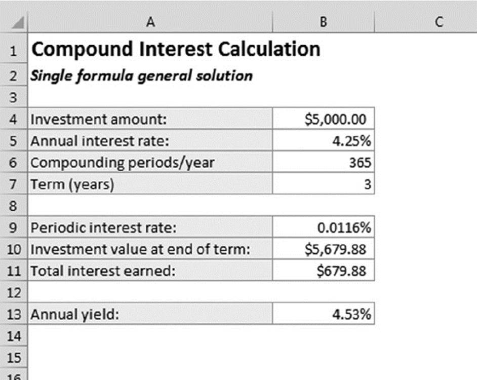
Figure 11.10 Calculating interest by using daily compounding.

Calculating interest with continuous compounding

The term continuous compounding refers to interest that is accumulated continuously. In other words, the investment has an infinite number of compounding periods per year. The following formula calculates the future value of a $5,000 investment at 4.25% compounded continuously for three years:

=5000*EXP(4.25&*3)

The formula returns $5,679.92, which is an additional $0.04 compared with daily compounding.

Note

You can calculate compound interest without using the FV function. The general formula to calculate compound interest is this:

Principal*(1+Periodic Rate)^Number of Periods

For example, consider a five-year, $5,000 investment that earns an annual interest rate of 4%, compounded monthly. The formula to calculate the future value of this investment follows:

=5000*(1+4&/12)^(12*5)

The Rule of 72

Need to make an investment decision but don’t have a computer handy? You can use the Rule of 72 to determine the number of years required to double your money at a particular interest rate using annual compounding. Just divide 72 by the interest rate. For example, consider a $10,000 investment at 4% interest. How many years will it take to turn that 10 grand into 20 grand? Take 72, divide it by 4, and you get 18 years. What if you can get a 5% interest rate? If so, you can double your money in a little over 14 years.

How accurate is the Rule of 72? The table that follows shows Rule of 72 estimated years versus the actual years for various interest rates. As you can see, this simple rule is remarkably accurate. However, for interest rates that exceed 30%, the accuracy drops off considerably.

The Rule of 72 also works in reverse. For example, if you want to double your money in six years, divide 6 into 72; you discover that you need to find an investment that pays an annual interest rate of about 12%.

Present value of a series of payments

The example in this section computes the present value of a series of future receipts, sometimes called an annuity.

A man gets lucky and wins the $1,000,000 jackpot in the state lottery. Lottery officials offer a choice:

§ Receive the $1 million as 20 annual payments of $50,000

§ In lieu of the $1 million, receive an immediate lump sum of $500,000

Ignoring tax implications, which is the better offer? In other words, what’s the present value of 20 years of annual $50,000 payments? And is the present value greater than the single lump sum payment of $500,000 (which has a present value of $500,000)?

The answer depends on making a prediction: if Mr. Lucky invests the money, what interest rate can be expected?

Assuming an expected 6% return on investment, calculate the present value of 20 annual $50,000 payments using this formula:

=PV(6&,20,50000,0,1)

The result is –$573,496.

Note

The present value is negative because it represents the amount Mr. Lucky would have to pay today to get those 20 years of payments at the stated interest rate. For this example, we can ignore the negative sign and treat it as positive value to be compared with the lump sum of $500,000.

What’s the decision? The lump sum amount would need to exceed $573,496 to make it a better deal for the lottery winner. The lump sum payout probably isn’t negotiable, so (based on an interest rate assumption of 6%) the 20 annual payments is a better deal for the lottery winner.

The PV calculation is sensitive to the interest rate assumption, which is often unknown. For example, if the lottery winner assumed an interest rate of 8% in the calculation, the present value of the 20 payments would be $490,907. Under this scenario, the lump sum would be a better choice.

In the extreme case, an interest rate of 0%, the PV calculates to $1,000,000. The lottery organization would have to pay the winner a lump sum of more than $1 million to make it more valuable than the payments spread over 20 years—not likely.

Future value of a series of deposits

Now consider another type of investment, one in which you make a regular series of deposits into an account. This type of investment is an annuity.

The worksheet functions discussed in the “Loan Calculations” section earlier in this chapter also apply to annuities, but you need to use the perspective of a lender, not a borrower. A simple example of this type of investment is a holiday club savings program offered by some banking institutions. A fixed amount is deducted from each of your paychecks and deposited into an interest-earning account. At the end of the year, you withdraw the money (with accumulated interest) to use for holiday expenses.

Suppose that you deposit $200 at the beginning of each month (for 12 months) into an account that pays 2.5% annual interest compounded monthly. The following formula calculates the future value of your series of deposits:

=FV(2.5&/12,12,-200,,1)

This formula returns $2,432.75, which represents the total of your deposits ($2,400.00) plus the interest ($32.75). The last argument for the FV function is 1, which means that you make payments at the beginning of the month. Figure 11.11 shows a worksheet set up to calculate annuities. Table 11.4 describes the contents of this sheet.

Table 11.4 The Annuity Calculator Worksheet

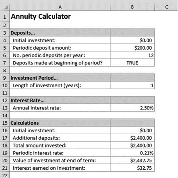
Figure 11.11 This worksheet contains formulas to calculate annuities.

On the Web

The workbook shown in Figure 11.11 is available at this book’s website. The file is named annuity calculator.xlsx.