Excel 2016 Formulas (2016)

PART III
Financial Formulas

Chapter 12
Discounting and Depreciation Formulas

In This Chapter

· Calculating the net present value of future cash flows

· Using cross-checking to verify results

· Calculating the internal rate of return

· Calculating the net present value of irregular cash flows

· Finding the internal rate of return on irregular cash flows

· Using the depreciation functions

The NPV (Net Present Value) and IRR (Internal Rate of Return) functions are perhaps the most commonly used financial analysis functions. This chapter provides many examples that use these functions for various types of financial analyses.

Using the NPV Function

The NPV function returns the sum of a series of cash flows, discounted to the present day using a single discount rate. The cash flow amounts can vary, but they must be at regular intervals (for example, monthly). The syntax for Excel’s NPV function is shown here; arguments in bold are required:

NPV(rate,value1,value2, …)

Cash inflows are represented as positive values, and cash outflows are negative values. The NPV function is subject to the same restrictions that apply to financial functions, such as PV, PMT, FV, NPER, and RATE (see Chapter 11, “Borrowing and Investing Formulas”).

If the discounted negative flows exceed the discounted positive flows, the function returns a negative amount. Conversely, if the discounted positive flows exceed the discounted negative flows, the NPV function returns a positive amount.

The rate argument is the discount rate—the rate at which future cash flows are discounted. It represents the rate of return that the investor requires. If NPV returns zero, it indicates that the future cash flows provide a rate of return exactly equal to the specified discount rate.

If the NPV is positive, it indicates that the future cash flows provide a better rate of return than the specified discount rate. The positive amount returned by NPV is the amount that the investor could add to the initial cash flow (called Point 0) to get the exact rate of return specified.

As you may have guessed, a negative NPV signifies that the investor does not get the required discount rate, often called a hurdle rate. To achieve the desired rate, the investor must reduce the initial cash outflow (or increase the initial cash inflow) by the amount returned by the negative NPV.

Note

The discount rate used must be a single effective rate for the period used for the cash flows. Therefore, if flows are set to monthly, you must use the monthly effective rate.

Definition of NPV

Excel’s NPV function assumes that the first cash flow is received at the end of the first period.

Warning

This assumption differs from the definition used by most financial calculators, and it is at odds with the definition used by institutions such as the Appraisal Institute of America (AIA). For example, the AIA defines NPV as the difference between the present value of positive cash flows and the present value of negative cash flows. If you use Excel’s NPV function without making an adjustment, the result does not adhere to this definition.

The point of an NPV calculation is to determine whether an investment will provide an appropriate return. The typical sequence of cash flows is an initial cash outflow followed by a series of cash inflows. For example, you buy a hot dog cart and some hot dogs (initial outflow) and spend the summer months selling them on a street corner (series of inflows). If you include the initial cash flow as an argument, NPV assumes the initial investment isn’t made right now but instead at the end of the first month (or some other time period).

Figure 12.1 shows three calculations using the same cash flows: a $20,000 initial outflow, a series of monthly inflows, and an 8% discount rate.

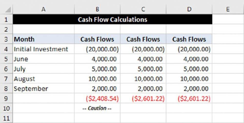
Figure 12.1 Three methods of computing NPV.

The formulas in row 9 are as follows:

B9: =NPV(8%,B4:B8)

C9: =NPV(8%,C5:C8)+C4

D9: =NPV(8%,D4:D8)*(1+8%)

The formula in B9 produces a result that differs from the other two. It assumes the $20,000 investment is made one month from now. There are applications where this is useful, but they rarely (if ever) involve an initial investment. The other two formulas answer the question of whether a $20,000 investment right now will earn 8%, assuming the future cash flows. The formulas in C9 and D9 produce the same result and can be used interchangeably.

NPV function examples

This section contains a number of examples that demonstrate the NPV function.

On the Web

All the examples in this section are available in the workbook net present value.xlsx at this book’s website.

Initial investment

Many NPV calculations start with an initial cash outlay followed by a series of inflows. In this example, the Time 0 cash flow is the purchase of a snowplow. Over the next ten years, the plow will be used to clear driveways and earn revenue. Experience shows that such a snowplow lasts 10 years. After that time, it will be broken down and worthless. Figure 12.2 shows a worksheet set up to calculate the NPV of the future cash flows associated with buying the plow.

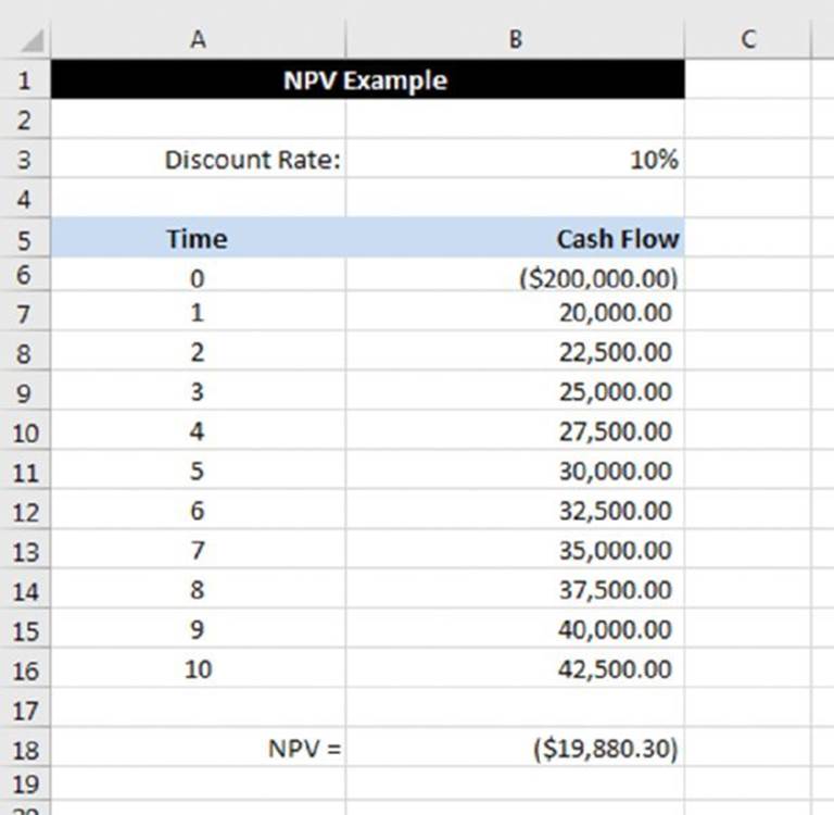
Figure 12.2 An initial investment returns positive future cash flows.

The NPV calculation in cell B18 uses the following formula, which returns –$19,880.30:

=NPV($B$3,B7:B16)+B6

The NPV is negative, so this analysis indicates that buying the snowplow is not a good investment. Here are several factors that influence the result:

§ First, a “good investment” is defined in the formula as one that returns 10%. If you can settle for a lesser return, lower the discount rate.

§ The future cash flows are generally (but not always) estimates. In this case, the potential plow owner assumes increasing revenue over the 10-year life of the equipment. Unless he has a 10-year contract to plow snow that sets forth the exact amounts to be received, the future cash flows are educated guesses at how much money he can make.

§ Finally, the initial investment plays a significant role in the calculation. If you can get the snowplow dealer to lower his price, the 10-year investment may prove worthwhile.

No initial investment

You can look at the snowplow example in a different way. In the previous example, you knew the cost of the snowplow and included that as the initial investment. The calculation determines whether the initial investment would produce a 10% return. You can also use NPV to tell what initial investment is required to produce the required return. That is, how much should you pay for the snowplow? Figure 12.3 shows the calculation of the NPV of a series of cash flows with no initial investment.

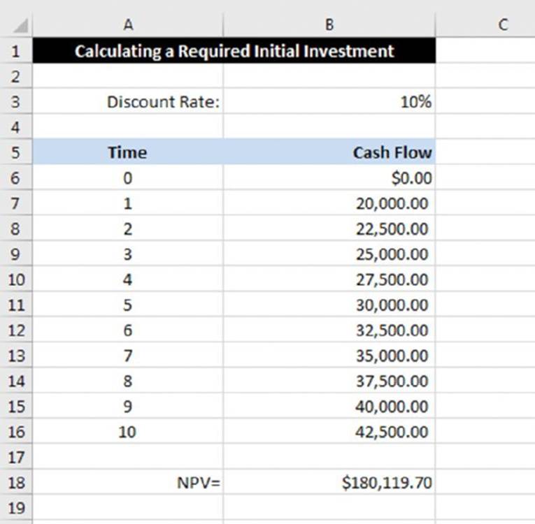
Figure 12.3 The NPV function can be used to determine the initial investment required.

The NPV calculation in cell B18 uses the following formula:

=NPV($B$3,B7:B16)+B6

If the potential snowplow owner can buy the snowplow for $180,119.70, it results in a 10% rate of return—assuming that the cash flow projections are accurate, of course.

Note

The formula adds the value in B6 to the end to be consistent with the formula from the previous example. Obviously, because the initial cash flow is zero, adding B6 is superfluous.

Initial cash inflow

Figure 12.4 shows an example in which the initial cash flow (the Time 0 cash flow) is an inflow. Like the previous example, this calculation returns the amount of an initial investment that is necessary to achieve the desired rate of return. In this example, however, the initial investment entitles you to receive the first inflow immediately.

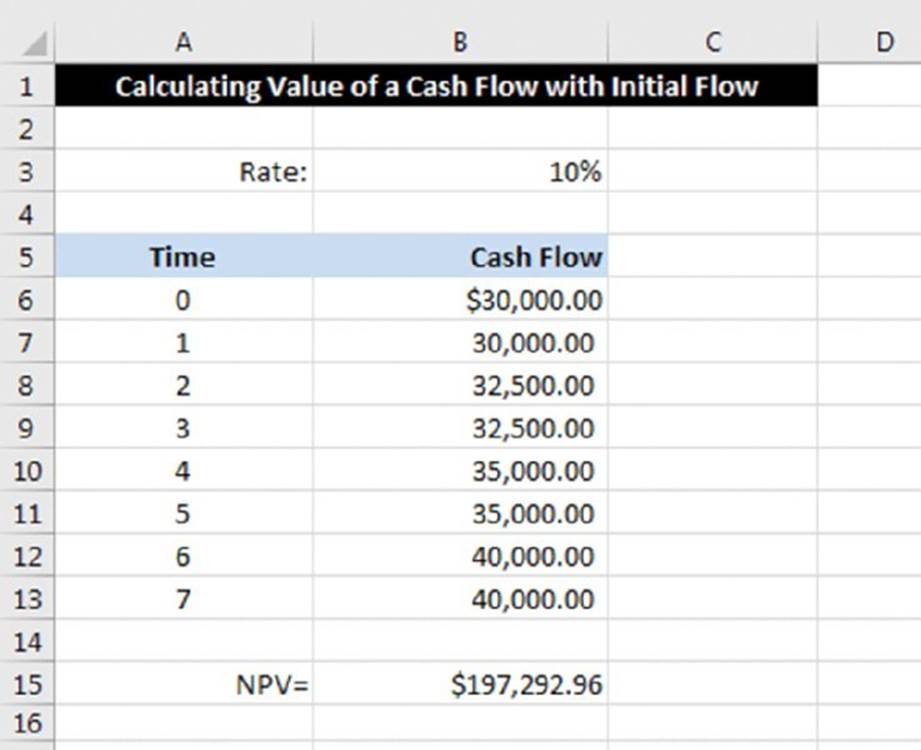
Figure 12.4 Some NPV calculations include an initial cash inflow.

The NPV calculation is in cell B15, which contains the following formula:

=NPV(B3,B7:B13)+B6

This example might seem unusual, but it is common in real estate situations in which rent is paid in advance. This calculation indicates that you can pay $197,292.96 for a rental property that pays back the future cash flows in rent. The first year’s rent, however, is due immediately. Therefore, the first year’s rent is shown at Time 0.

Terminal values

The previous example is missing one key element: namely, the disposition of the property after seven years. You can keep renting it forever, in which case you need to increase the number of cash flows in the calculation. Or you can sell it, as shown in Figure 12.5.

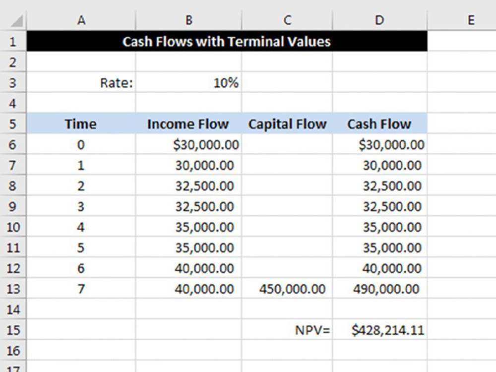
Figure 12.5 The initial investment may still have value at the end of the cash flows.

The NPV calculation in cell D15 follows:

=NPV(B3,D7:D13)+D6

In this example, the investor can pay $428,214.11 for the rental property, collect rent for seven years, sell the property for $450,000, and make 10% on his investment.

Initial and terminal values

This example uses the same cash flows as the previous example except that you know how much the owner of the investment property wants. It represents a typical investment example in which the aim is to determine if, and by how much, an asking price exceeds a desired rate of return, as you can see in Figure 12.6.

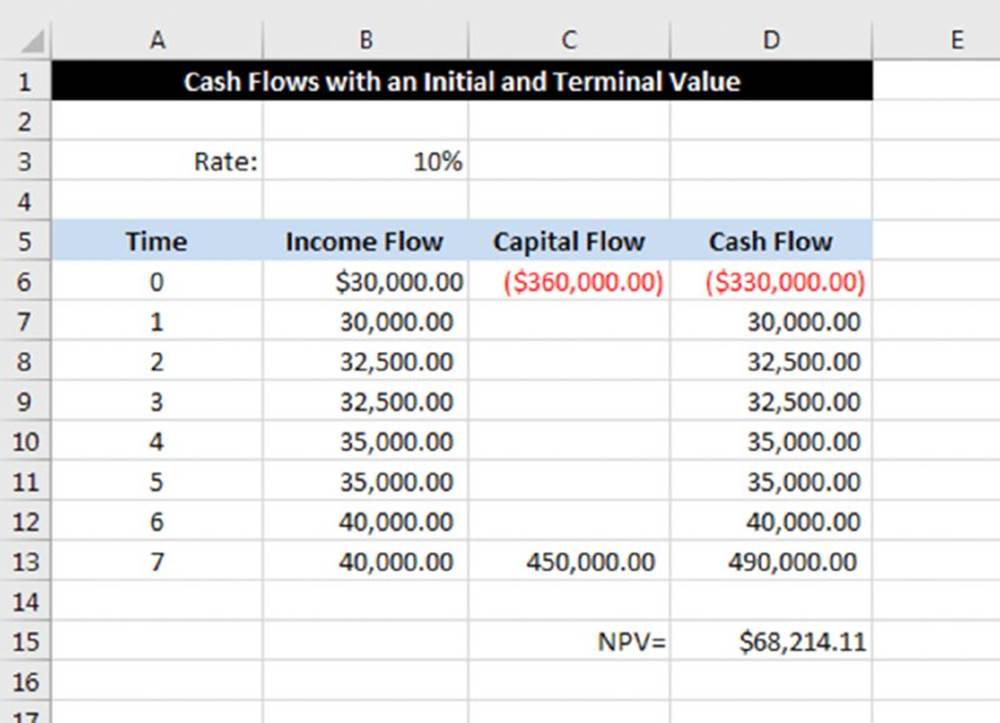
Figure 12.6 The NPV function can include an initial value and a terminal value.

The following formula indicates that at a $360,000 asking price, the discounted positive cash at the desired rate of return is $68,214.11:

=NPV(B3,D9:D15)+D8

The resulting positive NPV means that the investor can pay the asking price and make more than his desired rate of return. In fact, he can pay $68,214.11 more than the asking price and still meet his objective.

Future outflows

Although the typical investment decision may consist of an initial cash outflow resulting in periodic inflows, that’s certainly not always the case. The flexibility of NPV is that you can have varying amounts, both positive and negative, at all the points in the cash flow schedule.

In this example, a company wants to roll out a new product. It needs to purchase equipment for $475,000 and needs to spend another $225,000 to overhaul the equipment after five years. Also, the new product won’t be profitable at first but will be eventually.

Figure 12.7 shows a worksheet set up to account for all these varying cash flows. The formula in cell E18 is this:

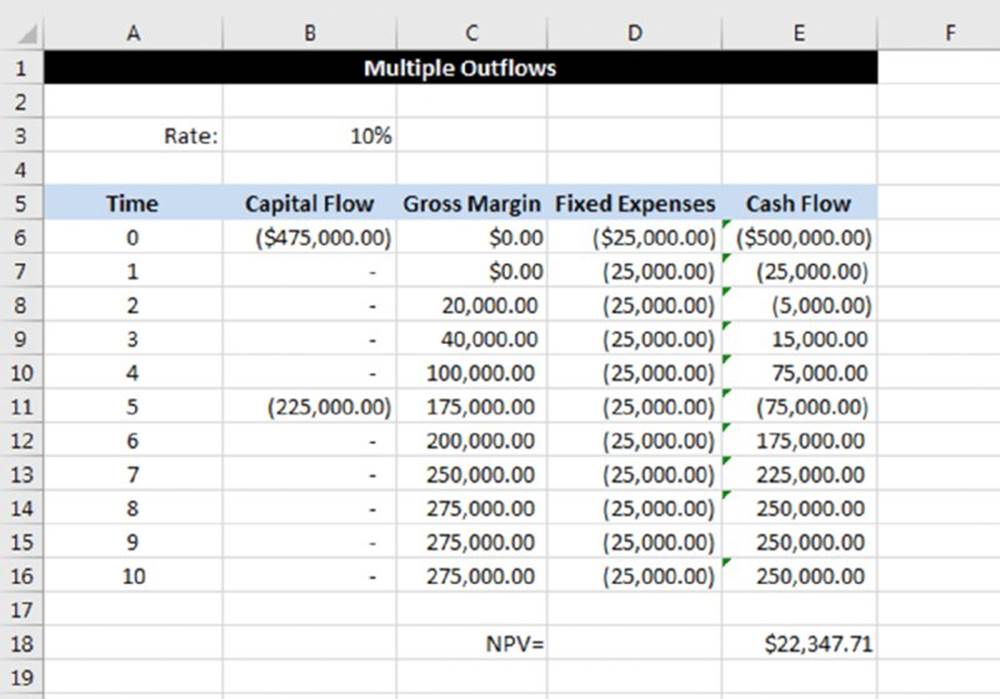
Figure 12.7 The NPV function can accept multiple positive and negative cash flows.

=NPV(B3,E7:E16)+E6

The positive NPV indicates that the company should invest in the equipment and start producing the new product. If it does, and the estimates of gross margin and expenses are accurate, the company will earn better than 10% on its investment.

Using the IRR Function

Excel’s IRR function returns the discount rate that makes the NPV of an investment zero. In other words, the IRR function is a special-case NPV.

The syntax of the IRR function follows:

IRR(range,guess)

Warning

The range argument must contain values. Empty cells are not treated as zero. If the range contains empty cells or text, the cells are ignored.

In most cases, the IRR can be calculated only by iteration. The guess argument, if supplied, acts as a “seed” for the iteration process. It has been found that a guess of –90% will almost always produce an answer. Other guesses, such as 0, usually (but not always) produce an answer.

An essential requirement of the IRR function is that there must be both negative and positive income flows. To get a return, there must be an outlay, and there must be a payback. There is no essential requirement for the outlay to come first. For a loan analysis using IRR, the loan amount is positive (and comes first), and the repayments that follow are negative.

The IRR is a powerful tool, and its uses extend beyond simply calculating the return from an investment. This function can be used in any situation in which you need to calculate a time- and data-weighted average return.

On the Web

The examples in this section are in a workbook named internal rate of return.xlsx, which is available at this book’s website.

Rate of return

This example sets up a basic IRR calculation (see Figure 12.8). An important consideration when calculating IRR is the payment frequency. If the cash flows are monthly, the IRR is monthly. In general, you want to convert the IRR to an annual rate. The example uses data validation in cell C3 to allow the user to select the type of flow (annual, monthly, daily, and so on) that displays in cell D3. That choice determines the appropriate interest conversion calculation; it also affects the labels in row 5, which contain formulas that reference the text in cell D3.

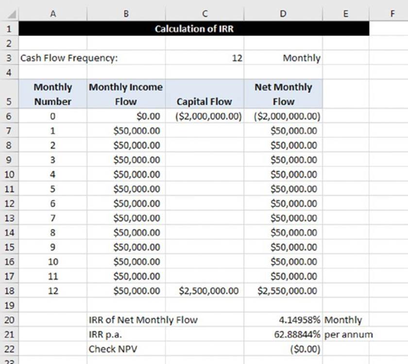
Figure 12.8 The IRR returns the rate based on the cash flow frequency and should be converted into an annual rate.

Cell D20 contains this formula:

=IRR(D6:D18,–90%)

Cell D21 contains this formula:

=FV(D20,C3,0,–1)–1

The following formula, in cell D22, is a validity check:

=NPV(D20,D7:D18)+D6

The IRR is the rate at which the discounting of the cash flow produces an NPV of zero. The formula in cell D22 uses the IRR in an NPV function applied to the same cash flow. The NPV discounting at the IRR (per month) is $0.00, so the calculation checks.

Geometric growth rates

You may have a need to calculate an average growth rate or average rate of return. Because of compounding, a simple arithmetic average does not yield the correct answer. Even worse, if the flows are different, an arithmetic average does not take these variations into account.

A solution uses the IRR function to calculate a geometric average rate of return. This is simply a calculation that determines the single percentage rate per period that exactly replaces the varying ones.

This example (see Figure 12.9) shows the IRR function being used to calculate a geometric average return based on index data (in column B). The calculations of the growth rate for each year are in column C. For example, the formula in cell C5 follows:

=(B5/B4)–1

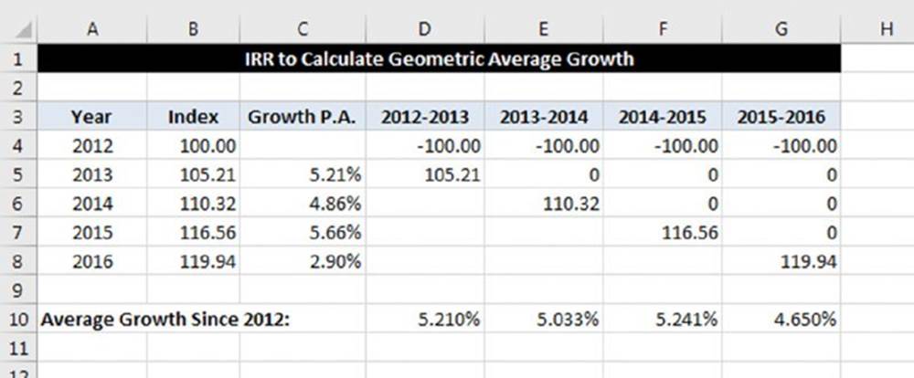
Figure 12.9 Using the IRR function to calculate geometric average growth.

The remaining columns show the geometric average growth rate between different periods. The formulas in row 10 use the IRR function to calculate the internal rate of return. For example, the formula in cell F10, which returns 5.241%, is this:

=IRR(F4:F8,–90%)

In other words, the growth rates of 5.21%, 4.86%, and 5.66% are equivalent to a geometric average growth rate of 5.241%.

The IRR calculation takes into account the direction of flow and places a greater value on the larger flows.

Checking results

Figure 12.10 shows a worksheet that demonstrates the relationship between IRR, NPV, and PV by verifying the results of some calculations. This verification is based on the definition of IRR: the rate at which the sum of positive and negative discounted flows is 0.

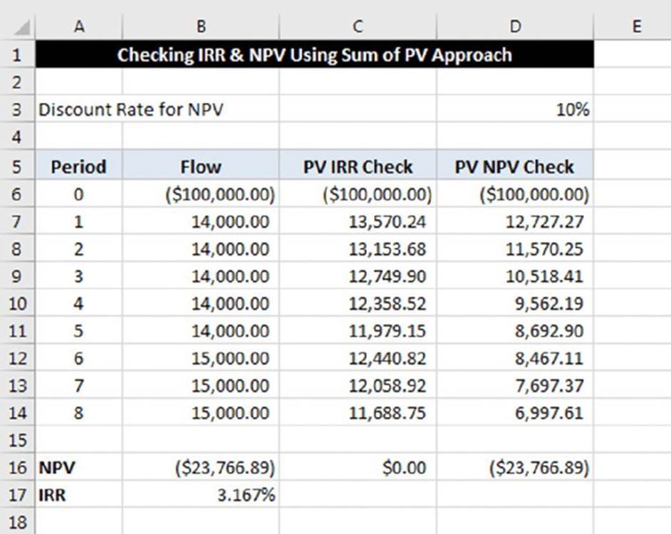
Figure 12.10 Checking IRR and NPV using the sum of PV approach.

The NPV is calculated in cell B16:

=NPV(D3,B7:B14)+B6

The internal rate of return is calculated in cell B17:

=IRR(B6:B14,–90%)

In column C, formulas calculate the present value. They use the IRR (calculated in cell B17) as the discount rate and use the period number (in column A) for the nper argument. For example, the formula in cell C6 follows:

=PV($B$17,A6,0,–B6)

The sum of the values in column C is 0, which verifies that the IRR calculation is accurate.

The formulas in column D use the discount rate (in cell D3) to calculate the present values. For example, the formula in cell D6 is this:

=PV($D$3,A6,0,–B6)

The sum of the values in column D is equal to the NPV.

For serious applications of NPV and IRR functions, it is an excellent idea to use this type of cross-checking.

Irregular Cash Flows

All the functions discussed so far—NPV, IRR, and MIRR—deal with cash flows that are regular. That is, they occur monthly, quarterly, yearly, or at some other periodic interval. Excel provides two functions for dealing with cash flows that don’t occur regularly: XNPV and XIRR.

Net present value

The syntax for XNPV follows:

XNPV(rate,values,dates)

The difference between XNPV and NPV is that XNPV requires a series of dates to which the values relate. In the example shown in Figure 12.11, the NPV of a series of irregular cash flows is found using XNPV.

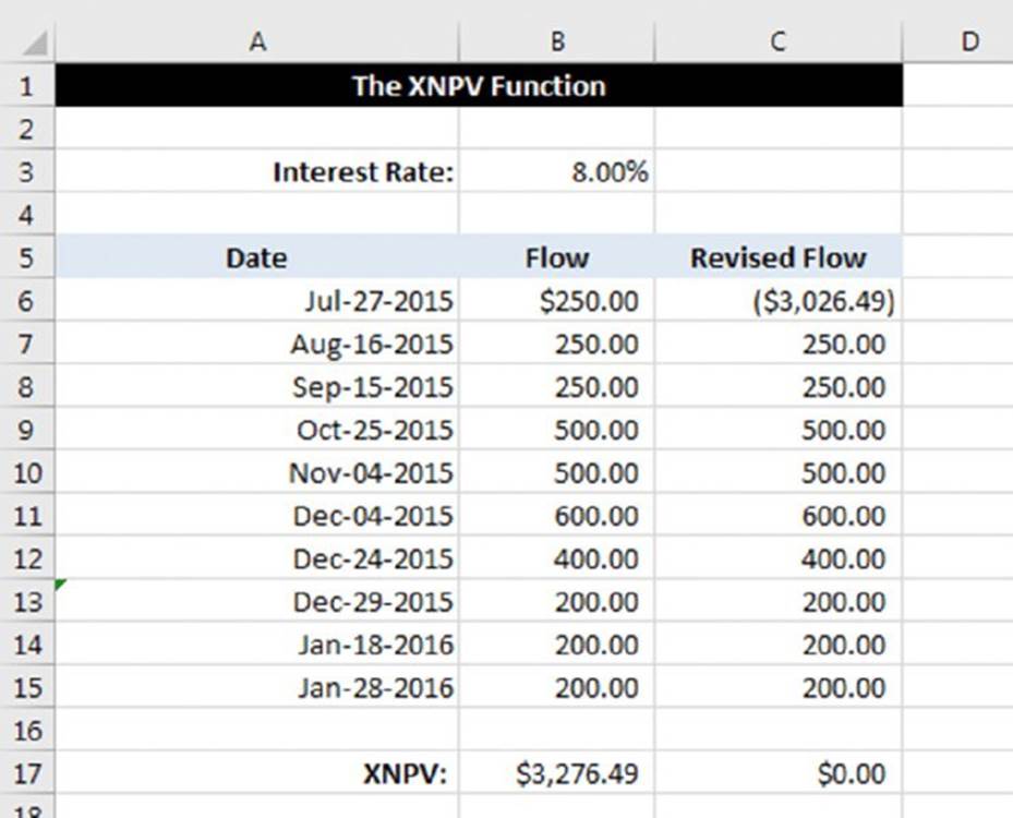
Figure 12.11 The XNPV function works with irregular cash flows.

On the Web

This book’s website contains the workbook irregular cash flows.xlsx, which contains all the examples in this section.

The formula in cell B17 is

=XNPV(B3,B6:B15,A6:A15)

Similar to NPV, the result of XNPV can be checked by duplicating the cash flows and netting the result with the first cash flow. The XNPV of the revised cash flows will be zero.

Note

Unlike the NPV function, XNPV assumes that the cash flows are at the beginning of each period instead of at the end. With NPV, we had to exclude the initial cash flow from the arguments and add it to the end of the formula. With XNPV, there is no need to do that.

Internal rate of return

The syntax for the XIRR function follows:

XIRR(value,dates,guess)

Just like XNPV, XIRR differs from its regular cousin by requiring dates. Figure 12.12 shows an example of computing the internal rate of return on a series of irregular cash flows.

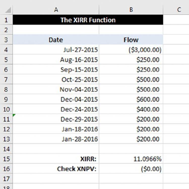
Figure 12.12 The XIRR function works with irregular cash flows.

The formula in B15 is:

=XIRR(B4:B13,A4:A13)

Warning

The XIRR function has the same problem with multiple rates of return as IRR. It expects that the cash flow changes signs only once: that is, goes from negative to positive or from positive to negative. If the sign changes more than once, it is essential that you plug the XIRR result back into an XNPV function to verify that it returns zero. Figure 12.12 shows such a verification, although the sign only changes once in that example.

Depreciation Calculations

Depreciation is an accounting concept whereby the value of an asset is expensed over time. Some expenditures affect only the current period and are expensed fully in that period. Other expenditures, however, affect multiple periods. These expenditures arecapitalized (made into an asset) and depreciated (written off a little each period). A forklift, for example, may be useful for five years. Expensing the full cost of the forklift in the year it was purchased would not put the correct cost into the correct years. Instead, the forklift is capitalized, and one-fifth of its cost is expensed in each year of its useful life.

On the Web

The examples in this section are available at this book’s website. The workbook is named depreciation.xlsx.

Table 12.1 summarizes Excel’s depreciation functions and the arguments used by each. For complete details, consult Excel’s Help system.

Table 12.1 Excel Depreciation Functions

* Arguments in brackets are optional.

The arguments for the depreciation functions are described as follows:

§ cost: Original cost of the asset.

§ salvage: Salvage cost of the asset after it has fully depreciated.

§ life: Number of periods over which the asset will depreciate.

§ period: Period in the life for which the calculation is being made. The VBD function uses two arguments: start period and end period.

§ month: Number of months in the first year; if omitted, Excel uses 12.

§ factor: Rate at which the balance declines; if omitted, it is assumed to be 2 (that is, double-declining).

§ no switch: TRUE or FALSE. Specifies whether to switch to straight-line depreciation when depreciation is greater than the declining balance calculation.

Figure 12.13 shows depreciation calculations using the SLN, DB, DDB, and SYD functions. The asset’s original cost, $10,000, is assumed to have a useful life of ten years, with a salvage value of $1,000. The range labeled Depreciation Amount shows the annual depreciation of the asset. The range labeled Value of Asset shows the asset’s depreciated value over its life.

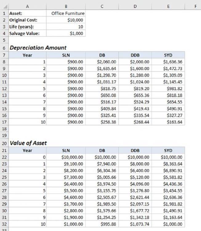
Figure 12.13 A comparison of four depreciation functions.

Figure 12.14 shows a chart that graphs the asset’s value. As you can see, the SLN function produces a straight line; the other functions produce curved lines because the depreciation is greater in the earlier years of the asset’s life.

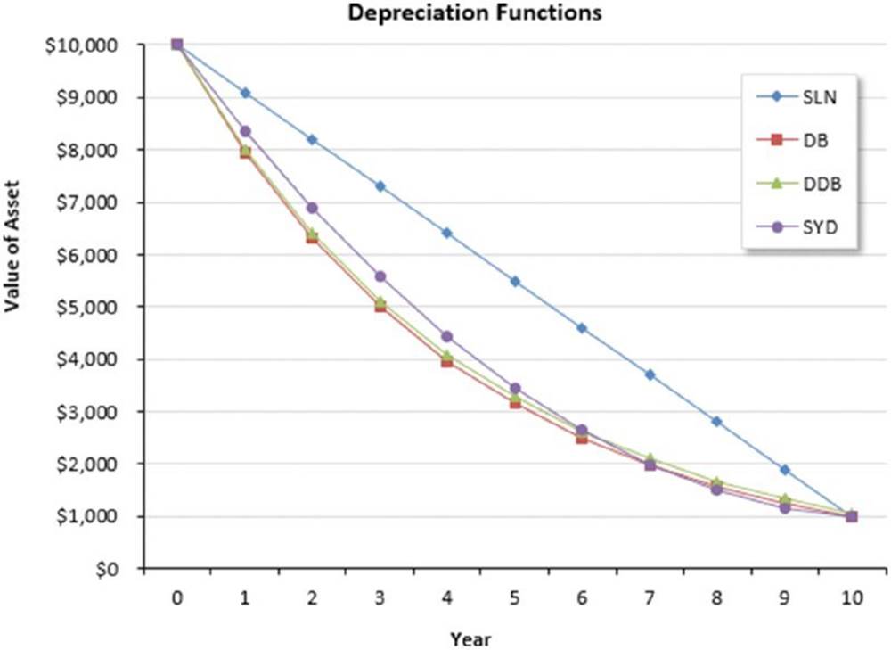
Figure 12.14 This chart shows an asset’s value over time, using four depreciation functions.

The VDB (variable declining balance) function is useful if you need to calculate depreciation for multiple periods, such as when you need to figure accumulated depreciation on an asset that has been sold. Figure 12.15 shows a worksheet set up to calculate the gain or loss on the sale of some office furniture. The formula in cell B12 is this:

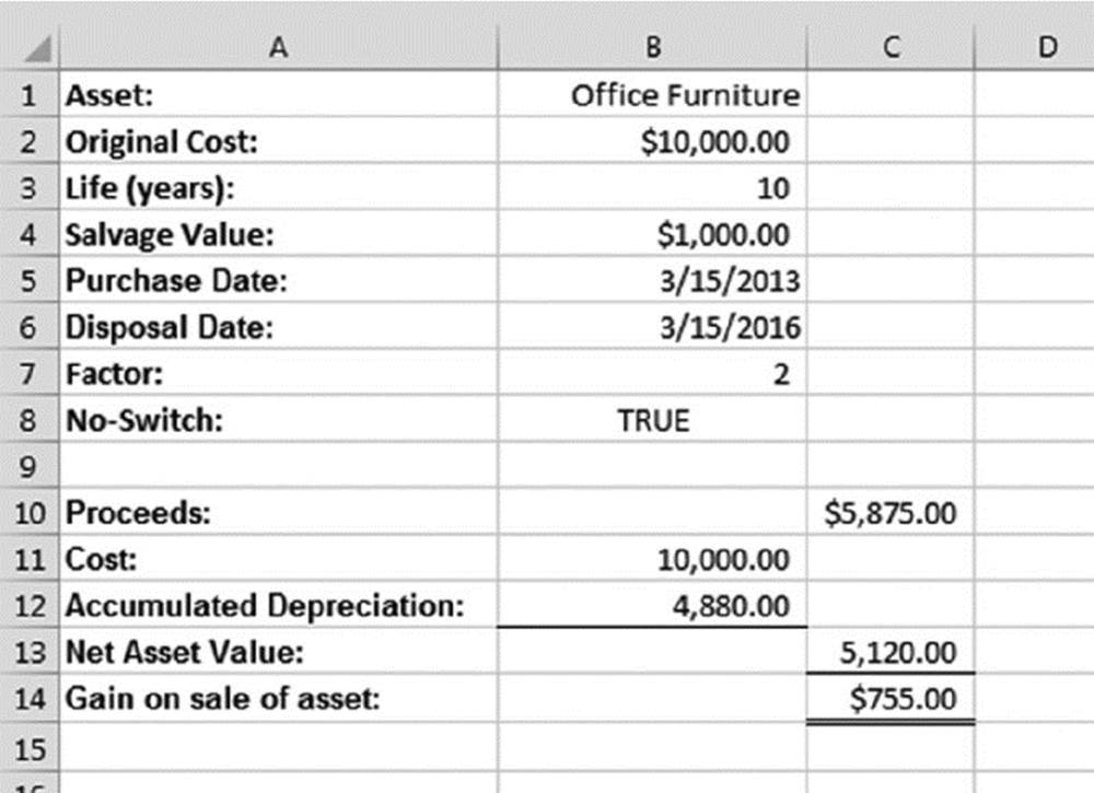
Figure 12.15 Using the VDB function to calculate accumulated depreciation.

=VDB(B2,B4,B3,0,DATEDIF(B5,B6,"y"),B7,B8)

The formula computes the depreciation taken on the asset from the date it was purchased until the date it was sold. The DATEDIF function is used to determine how many years the asset has been in service.