Excel 2016 Formulas (2016)

PART III
Financial Formulas

Chapter 13
Financial Schedules

In This Chapter

· Setting up a basic amortization schedule

· Setting up a dynamic amortization schedule

· Evaluating loan options with a data table

· Creating two-way data tables

· Creating financial statements

· Understanding credit card repayment calculations

· Calculating and evaluating financial ratios

· Creating indices

This chapter, which makes use of much of the information contained in the two previous chapters, contains helpful examples of a variety of financial calculations.

Creating Financial Schedules

Financial schedules present financial information in many different forms. Some present a summary of information, such as a profit and loss statement. Others present a detailed list, such as an amortization schedule, which schedules the payments for a loan.

Financial schedules can be static or dynamic. Static schedules generally use a few Excel functions but mainly exist in Excel to take advantage of its grid system, which lends itself well for formatting schedules. Dynamic schedules, on the other hand, usually contain an area for user input. A user can change certain input parameters and affect the results.

The sections that follow demonstrate summary and detail schedules, as well as static and dynamic schedules.

Creating Amortization Schedules

In its simplest form, an amortization schedule tracks the payments (including interest and principal components) and the loan balance for a particular loan. This section presents several examples of amortization schedules.

A simple amortization schedule

This example uses a simple loan to demonstrate the basic concepts involved in creating a schedule. Refer to the worksheet in Figure 13.1. Notice that rows 19 through 370 are hidden, so only the first four payments and last four payments are visible.

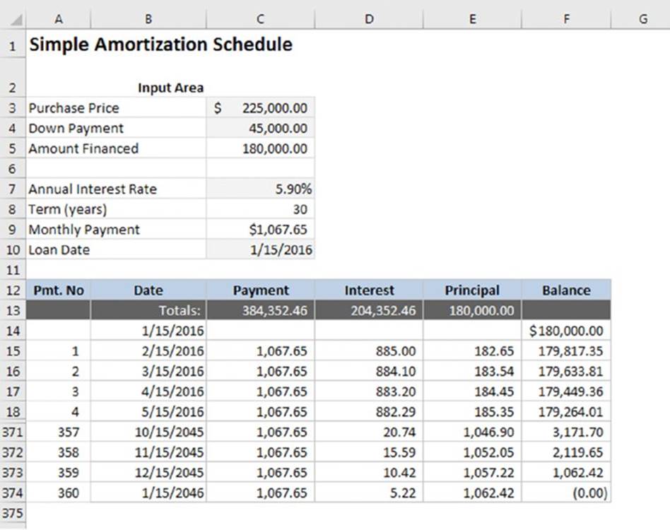
Figure 13.1 A simple amortization schedule.

On the Web

All the examples in this section are available at this book’s website in the workbook loan amortization.xlsx.

User input section

The area above the schedule contains cells for user input and for intermediate calculations. The user input cells are shaded, making it easy to distinguish between cells that can be changed and cells that are calculated by formulas.

The user can enter the purchase price and the down payment. The amount financed is calculated for use in the amortization calculation. Here’s the formula in cell B5:

=Purchase_Price–Down_Payment

Tip

Names are used to make the formulas more readable. More information on named cells and ranges is in Chapter 3, “Working with Names.”

The other calculation necessary to complete the schedule is the monthly payment. Here’s the formula in B9:

=-PMT(Rate/12,Term*12,Amount_Financed)

The PMT function is used to determine the monthly payment amount. The rate (B7) is divided by 12, and the term (B8) is multiplied by 12, so that the arguments are on a monthly basis. This ensures that the result of PMT is also on a monthly basis.

Because this is a simple amortization schedule, the loan term is fixed at 30 years. Using a different term requires adding or deleting rows of formulas and changing the summary formulas.

Summary information

The first line of the schedule (row 13) contains summary formulas. Placing the summary information above the schedule eliminates the need to scroll to the end of the worksheet.

In this example, only the totals are shown. However, you can include subtotals by year, quarter, or any other interval you like. The formula in C13 sums 360 cells and is copied across the next two columns:

=SUM(C15:C374)

The schedule

The schedule starts in row 14, which shows the loan date and the amount financed (the beginning balance). The first payment is made exactly one month after the loan is initiated. The first payment row (row 15) and all subsequent rows contain the same formulas, which we describe later.

The Payment column simply references the Monthly_Payment cell in the user input section.

The Interest column computes a monthly interest based on the previous loan balance. The formula in D15 is this:

=F14*(Rate/12)

The previous balance, in cell F14, is multiplied by the annual interest rate, which is divided by 12. The annual interest rate is in cell B7, named Rate.

Whatever portion of the payment doesn’t go toward interest goes toward reducing the principal balance. The formula in E15 is this:

=C15–D15

Finally, the balance is updated to reflect the principal portion of the payment. The formula in E15 is this:

=F14–E15

Loan amortization schedules are self-checking. If everything is set up correctly, the final balance at the end of the term is 0 (or close to 0, given rounding errors). Another check is to add all the monthly Principal components. The sum of these values should equal the original loan amount.

Limitations

This type of schedule is suitable for loans that will likely never change. It can be set up one time and referred to throughout the life of the loan. Further, you can copy it to create a new loan with just a few adjustments. However, this schedule lacks flexibility:

§ The payment is computed and applied every month but cannot account for overpayments. Borrowers often pay an additional amount that is applied to the principal, thereby reducing the pay-off period.

§ Many loans have variable interest rates, and this schedule provides no way to adjust the interest rate per period.

§ The schedule has a fixed term of 30 years. A loan with a shorter or longer term would require that formulas be deleted or added to compensate.

In the next section, we address some of the flexibility issues and create a more dynamic amortization schedule.

A dynamic amortization schedule

The example in this section builds on the previous example. Figure 13.2 shows part of a loan amortization schedule that allows the user to define input parameters beyond the loan amount and rate.

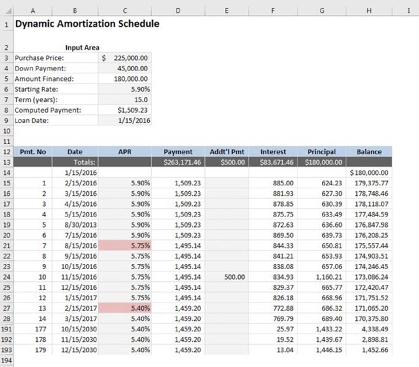
Figure 13.2 A dynamic amortization schedule.

The first difference you’ll notice is that this schedule has two additional columns: APR and Addt’l Pmt. These columns are shaded, which indicates that the values can be changed.

User input section

This schedule has a few changes in the Input Area at the top. The interest rate is labeled Starting Rate, and the payment is labeled Computed Payment, indicating that they are subject to change. Also, the user can now specify the term of the loan.

Summary information

Because the user can now change the term and make additional payments, the maturity date isn’t always fixed. The formulas are set up for a maximum of 360 payments, but not all these rows need to be summed. For the summary information, you want to sum only the rows up until the loan is paid off. The formula in D13 follows:

=SUMIF($H15:$H374,">=–1",D15:D374)

After the Balance in column H is zero, the amortization is complete. This SUMIF function sums only those payments up until that point. This formula is copied across the next three columns. Note that the condition is “greater than or equal to –1.” This handles the situation in which the final balance isn’t exactly zero (but close to it).

Changing the APR

If the interest rate changes, the user can enter the new rate in the APR column. That new rate is in effect until a different rate is entered.

The formula in cell C15 retrieves the Starting_Rate value from the input area. The formula in cell C16, and copied down, is this:

=C15

If a new rate is entered, it overwrites the formula, and that new rate is propagated down the column. The effect is that the new rate is in effect for all subsequent payments—at least until it changes again.

In Figure 13.2, the rate was changed to 5.75% beginning with the seventh payment. The lower rate also affected the payments. The rate changed again beginning with the thirteenth payment, and again the payment amount was adjusted.

Note

We used conditional formatting for the cells in the APR column to make the rate changes stand out.

When the APR is changed, the payment amount is adjusted. The loan is essentially reamortized for the remaining term, using the new interest rate. Here’s the formula in cell D16:

=IF(C16<>C15,–PMT(C16/12,(Term*12)–A15,H15),D15)

This formula checks the value in the APR column. If it’s different from the APR in the previous row, the PMT function calculates the new payment. If the APR hasn’t changed, the previous payment is returned.

Handling additional payments

If additional payments are made, they are entered in column E. In Figure 13.2, an additional payment of $500 was applied to the tenth payment. Extra payments are applied to the principal.

The formula in cell G15 (and copied down) calculates the principal portion of the payment (and additional payment, if made):

=(D15–F15)+E15

Finishing touches

Because the loan term is specified by the user, we used conditional formatting to hide the rows that extend beyond the specified term.

All the cells in the schedule, starting in row 15, have conditional formatting applied to them. If column G of the row above is zero or less, both the background color and the font color are white, rendering them invisible.

To apply conditional formatting, select the range A15:H374 and choose the Home ➜ Styles ➜ Conditional Formatting command. Add a formula rule with this formula:

=$H15<0

Cross-Ref

For more information on conditional formatting, see Chapter 19, “Conditional Formatting.”

Credit card calculations

Another type of loan amortization schedule is for credit card loans. Credit cards are different because the minimum payment varies, based on the balance. You could use the method in which the payments are entered directly into the schedule. When the payments are different every time, however, the schedule loses its value as a predictor or planner. Here, we describe a schedule that can predict the payments of a credit card loan.

Credit card calculations represent several nonstandard problems. Excel’s financial functions (PV, FV, RATE, and NPER) require that the regular payments are at a single level. In addition, the PMT function returns a single level of payments. With IRR and NPV analysis, the user inserts the varying payments into a cash flow.

Credit card companies calculate payments based on the following relatively standard set of criteria:

§ A minimum payment is required. For example, a credit card account might require a minimum monthly payment of $25.

§ The payment must be at least equal to a base percentage of the debt. Usually, the payment is a percentage of the balance but not less than a specified amount.

§ The payment is rounded, usually to the nearest $0.05.

§ Interest is invariably quoted at a given rate per month.

Figure 13.3 shows a worksheet set up to calculate credit card payments.

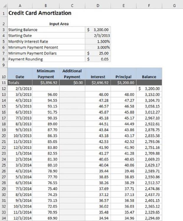
Figure 13.3 Calculating a credit card payment schedule.

The formula for the minimum payment is rather complicated—just like the terms of a credit card. This example uses a minimum payment amount of $25 or 3% of the balance, whichever is larger. This small minimum payment results in a long payback period. If this borrower ever hopes to pay off that balance in a reasonable amount of time, he needs to use that additional payment column.

The minimum payment formula, such as the one in B13, follows:

=MIN(F12+D13,MROUND(MAX(MinDol,ROUND(MinPct*F12,2)),PayRnd))

From the inside out: the larger of the minimum dollar amounts and the minimum percent are calculated. The result is rounded to the nearest five cents. This rounded amount is then compared with the outstanding balance (plus interest), and the lesser of the two is used.

Of course, things get much more complicated when additional charges are made. In such a case, the formulas need to account for “grace periods” for purchases (but not cash withdrawals). A further complication is that interest is calculated on the daily outstanding balance at the daily effective equivalent of the quoted rate.

Summarizing Loan Options Using a Data Table

If you’re faced with making a decision about borrowing money, you have to choose between many variables, not the least of which is the interest rate. Fortunately, Excel’s data table feature can help by summarizing the results of calculations using different inputs.

On the Web

The workbook loan data tables.xlsx contains the examples in this section and can be found at this book’s website.

The data table feature is one of Excel’s most under-used tools. A data table is a dynamic range that summarizes formula cells for varying input cells. You can create a data table fairly easily, but it has some limitations. In particular, a data table can deal with only one or two input cells at a time. This limitation becomes clear as you view the examples.

Creating a one-way data table

A one-way data table shows the results of any number of calculations for different values of a single input cell. Figure 13.4 shows the general layout for a one-way data table.

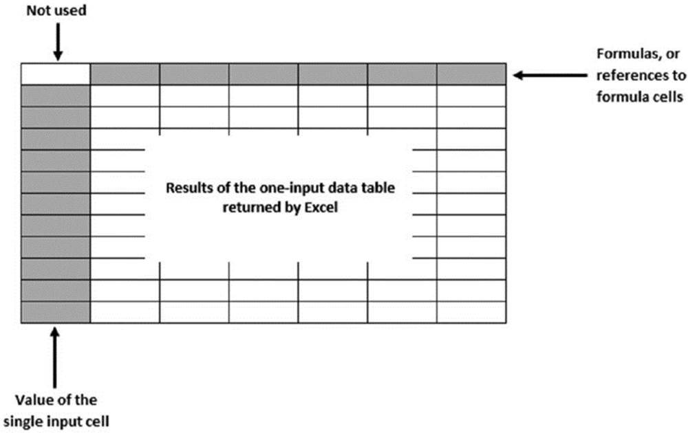
Figure 13.4 The layout for a one-way data table.

Figure 13.5 shows a one-way data table (in D2:G9) that displays three calculations (payment amount, total payments, and total interest) for a loan, using eight interest rates ranging from 6.75% to 8.50%. In this example, the input cell is cell B2. Note that the range E1:G1 is not part of the data table. These cells contain descriptive labels.

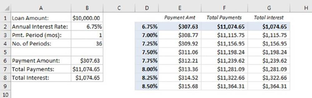
Figure 13.5 Using a one-way data table to display three loan calculations for various interest rates.

To create this one-way data table, follow these steps:

1. In the first row of the data table, enter the formulas that returns the results.

The interest rate varies in the data table, but it doesn’t matter which interest rate you use for the calculations as long as the calculations are correct. In this example, the formulas in E2:G2 contain references to other formulas in column B:

E2: =B6

F2: =B7

G2: =B8

2. In the first column of the data table, enter various values for a single input cell.

In this example, the input value is an interest rate, and the values for various interest rates appear in D2:D9. Note that the first row of the data table (row 2) displays the results for the first input value (in cell D2).

3. Select the range that contains the entries from the previous steps.

In this example, select D2:G9.

4. Choose Data➜ Forecast➜ What-If Analysis➜ Data Table.

Excel displays the Data Table dialog box, as shown in Figure 13.6.

5. For the Column Input Cell field, specify the formula cell that corresponds to the input variable.

In this example, the Column Input Cell is B2.

6. Leave the Row Input Cell field empty. Then click OK.

Excel inserts an array formula that uses the TABLE function with a single argument.

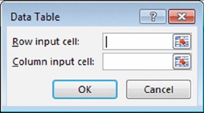
Figure 13.6 The Data Table dialog box

Note that the array formula is not entered into the entire range that you selected in step 3. The first column and the first row of your selection are not changed.

Creating a two-way data table

A two-way data table shows the results of a single calculation for different values of two input cells. Figure 13.7 shows the general layout of a two-way data table.

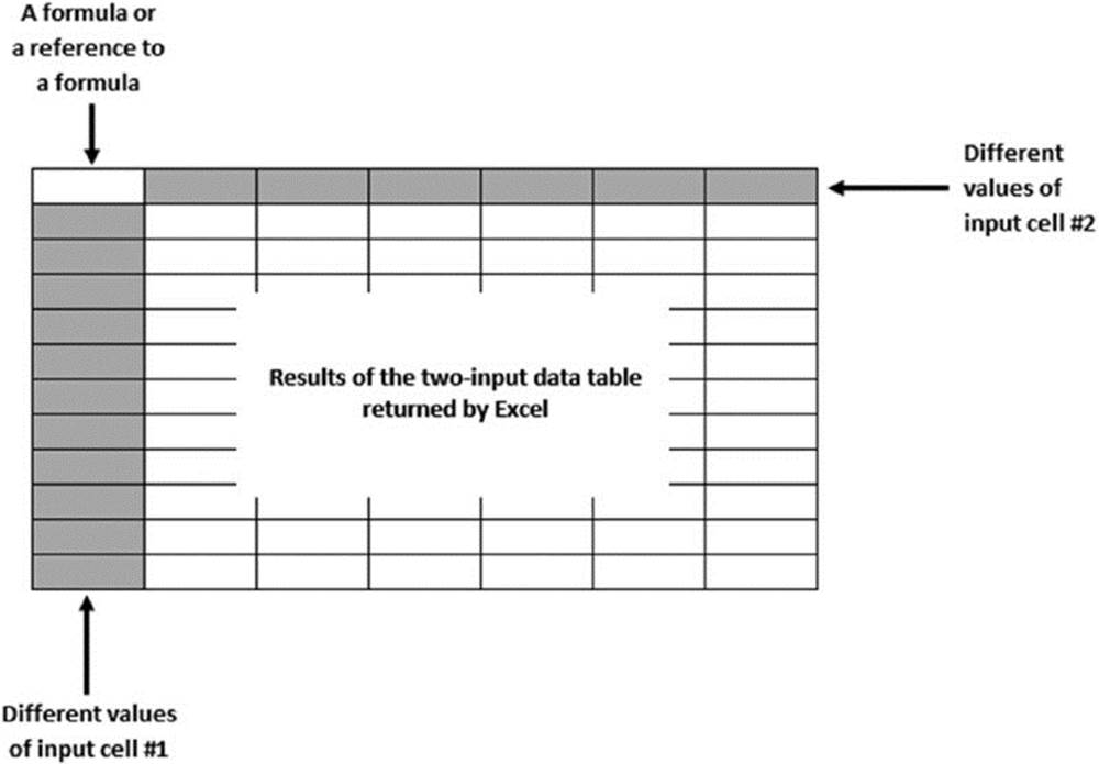
Figure 13.7 The structure for a two-way data table.

Figure 13.8 shows a two-way data table (in B7:J16) that displays a calculation (payment amount) for a loan, using eight interest rates and nine loan amounts.

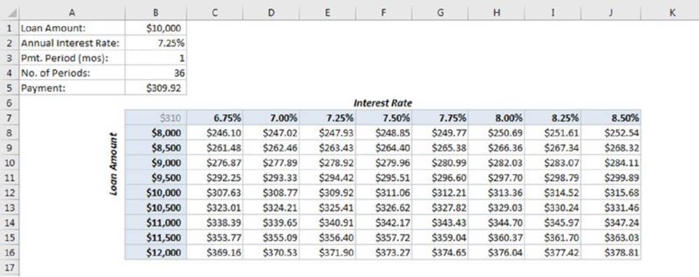
Figure 13.8 Using a two-way data table to display payment amounts for various loan amounts and interest rates.

To create this two-way data table, follow these steps:

1. Enter a formula that returns the results that you want to use in the data table.

In this example, the formula in cell B7 is a simple reference to cell B5, which contains the payment calculation:

=B5

2. Enter various values for the first input in successive columns of the first row of the data table.

In this example, the first input value is interest rate, and the values for various interest rates appear in C7:J7.

3. Enter various values for the second input cell in successive rows of the first column of the data table.

In this example, the second input value is the loan amount, and the values for various loan amounts are in B8:B16.

4. Select the range that contains the entries from the preceding steps.

For this example, select B7:J16.

5. Choose Data ➜ Forecast ➜ What-If Analysis ➜ Data Table.

Excel displays the Data Table dialog box.

6. For the Row Input Cell field, specify the cell reference that corresponds to the first input cell.

In this example, the Row Input Cell is B2.

7. For the Column Input Cell field, specify the cell reference that corresponds to the second input cell.

In this example, the Column Input Cell is B1.

8. Click OK.

Excel inserts an array formula that uses the TABLE function with two arguments.

After you create the two-way data table, you can change the formula in the upper-left cell of the data table. In this example, you can change the formula in cell B7 to

=PMT(B2*(B3/12),B4,–B1)*B4–B1

This causes the TABLE function to display total interest rather than payment amounts.

Tip

If you find that using data tables slows down the calculation of your workbook, choose Formulas ➜ Calculation ➜ Calculation Options ➜ Automatic Except for Data Tables. Then you can recalculate by pressing F9.

Financial Statements and Ratios

Many companies use Excel to evaluate their financial health and report financial results. Financial statements and financial ratios are two types of analyses a company can use to accomplish those goals. Excel is well suited for financial statements because its grid layout allows for easy adjustment of columns. Ratios are simple financial calculations—something Excel was designed for.

Basic financial statements

Financial statements summarize the financial transactions of a business. The two primary financial statements are the balance sheet and the income statement:

§ The balance sheet reports the state of a company at a particular moment in time. It shows the following:

· Assets: What the company owns

· Liabilities: What the company owes

· Equity: What the company is worth

§ The income statement summarizes the transactions of a company over a certain period of time, such as a month, quarter, or year.

§ A typical income statement reports the sales, costs, and net income (or loss) of the company.

Converting trial balances

Most accounting software produces financial statements for you. However, many of those applications do not give you the flexibility and formatting options that you have in Excel. One way to produce your own financial statements is to export the trial balance from your accounting software package and use Excel to summarize the transactions for you. Figure 13.9 shows part of a trial balance, which lists all the accounts and their balances.

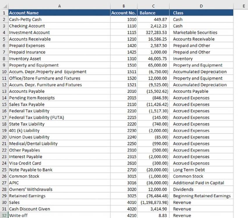
Figure 13.9 A trial balance lists all accounts and balances.

Figure 13.10 shows a balance sheet that summarizes the balance sheet accounts from the trial balance.

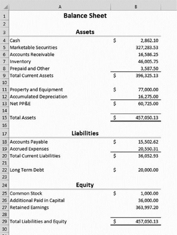
Figure 13.10 A balance sheet summarizes certain accounts.

The Class column of the trial balance is used to classify that account on the balance sheet or income statement. The formula in cell B4 on the balance sheet follows:

=SUMIF(Class,A4,Balance)

On the Web

The file financial statements.xlsx contains all the examples in this chapter and can be found at this book’s website.

For all the accounts on the trial balance whose class equals Cash, their total is summed here. The formula is repeated for every financial statement classification on both the balance sheet and the income statement. For classifications that typically have a credit balance—such as liabilities, equity, and revenue—the formula starts with a negative sign. Here’s the formula for Accounts Payable, cell B18:

=-SUMIF(Class,A18,Balance)

The account that ties the balance sheet and income statement together is Retained Earnings. Figure 13.11 shows an income statement that includes a statement of retained earnings at the bottom.

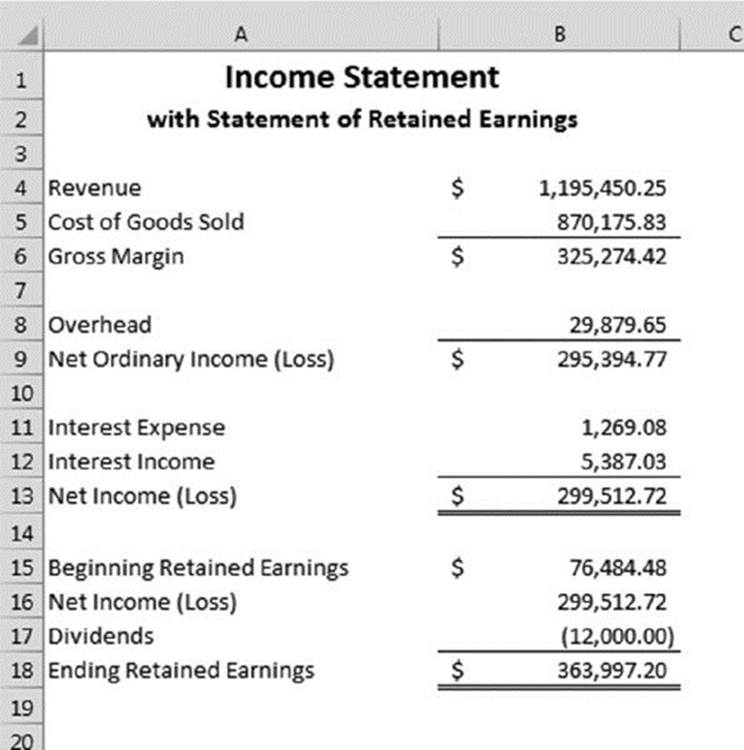
Figure 13.11 The income statement can include a statement of retained earnings.

The Retained Earnings classification on the balance sheet refers to the Ending Retained Earnings classification on the income statement. Ending Retained Earnings is computed by taking Beginning Retained Earnings, adding net income (or subtracting net loss), and subtracting dividends.

Finally, the balance sheet must be in balance: hence, the name. Total assets must equal total liabilities and equity. This error-checking formula is used in cell B31 on the balance sheet:

=IF(ABS(B29–B15)>0.01,"Out of Balance","")

If the difference between assets and liabilities and equity is more than a penny, an error message is displayed below the schedule; otherwise, the cell appears blank. The ABS function is used to check for assets being more or less than liabilities and equity. Because the balance sheet is in balance, the formula returns an empty string.

Common size financial statements

Comparing financial statements from different companies can be difficult. One such difficulty is comparing companies of different sizes. A small retailer might show $1 million in revenue, but a multinational retailer might show $1 billion. The sheer scale of the numbers makes it difficult to compare the health and results of operations of these very different companies.

Common size financial statements summarize accounts relative to a single number. For balance sheets, all entries are shown relative to total assets. For the income statement, all entries are shown relative to total sales. Figure 13.12 shows a common size income statement.

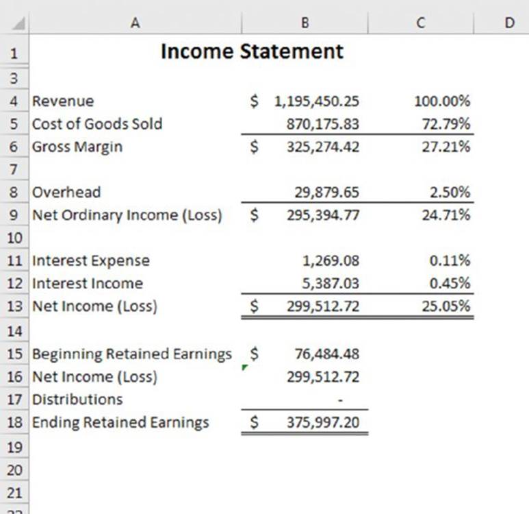
Figure 13.12 Entries on a common size income statement are shown relative to revenue.

The formula in cell C4 follows:

=B4/$B$4

The denominator is absolute with respect to both rows and columns so that when this formula is copied to other areas of the income statement, it shows the percentage of revenue. To display only the percentage figures, you can hide column B.

Ratio analysis

Financial ratios are calculations that are derived from the financial statements and other financial data to measure various aspects of a company. They can be compared with other companies or to industry standards. This section demonstrates how to calculate several financial ratios. See Figure 13.13

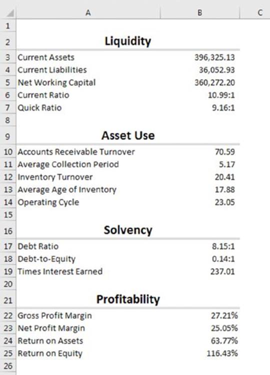
Figure 13.13 Various financial ratio calculations.

Liquidity ratios

Liquidity ratios measure a company’s ability to pay its bills in the short term. Poor liquidity ratios may indicate that the company has a high cost of financing or is on the verge of bankruptcy.

Net working capital is computed by subtracting current liabilities from current assets:

=Total_Current_Assets–Total_Current_Liabilities

Current assets are turned into cash within one accounting period (usually one year). Current liabilities are debts that will be paid within one period. A positive number here indicates that the company has enough assets to pay for its short-term liabilities.

The current ratio is a similar measure that divides current assets by current liabilities:

=Total_Current_Assets/Total_Current_Liabilities

When this ratio is greater than 1:1, it’s the same as when net working capital is positive.

The final liquidity ratio is the quick ratio. Although the current ratio includes assets, such as inventory and accounts receivable that will be converted into cash in a short time, the quick ratio includes only cash and assets that can be converted into cash immediately.

=(Cash+Marketable_Securities)/Total_Current_Liabilities

A quick ratio greater than 1:1 indicates that the company can pay all its short-term liabilities right now.

Tip

The following custom number format can be used to format the result of the current ratio and the quick ratio:

0.00":1"_)

Asset use ratios

Asset use ratios measure how efficiently a company is using its assets: that is, how quickly the company is turning its assets back into cash. The accounts receivable turnover ratio divides sales by average accounts receivable:

=Revenue/((Account_Receivable+LastYear_Accounts_Receivable)/2)

Accounts receivable turnover is then used to compute the average collection period:

=365/Accounts_receivable_turnover

The average collection period is generally compared against the company’s credit terms. If the company allows 30 days for its customers to pay and the average collection period is greater than 30 days, it can indicate a problem with the company’s credit policies or collection efforts.

The efficiency with which the company uses its inventory can be similarly computed. Inventory turnover divides cost of sales by average inventory:

=Cost_of_Goods_Sold/((Inventory+LastYear_Inventory)/2)

The average age of inventory tells how many days’ inventory is in stock before it is sold:

=365/Inventory_turnover

By adding the average collection period to the average age of inventory, the total days to convert inventory into cash can be computed. This is the operating cycle and is computed as follows:

=Average_collection_period+Average_age_of_inventory

Solvency ratios

Whereas liquidity ratios compute a company’s ability to pay short-term debt, solvency ratios compute its ability to pay long-term debt. The debt ratio compares total assets with total liabilities:

=Total_Assets/(Total_Current_Liabilities+Long_Term_Debt)

The debt-to-equity ratio divides total liabilities by total equity. It’s used to determine whether a company is primarily equity financed or debt financed:

=(Total_Current_Liabilities+Long_Term_Debt)/

(Common_Stock+Additional_Paid_in_Capital+Retained_Earnings)

The times interest earned ratio computes how many times a company’s profit would cover its interest expense:

=(Net_Income__Loss+Interest_Expense)/Interest_Expense

Profitability ratios

As you might guess, profitability ratios measure how much profit a company makes. Gross profit margin and net profit margin can be seen on the earlier common size financial statements because they are both ratios computed relative to sales. The formulas for gross profit margin and net profit margin follow:

=Gross_Margin/Revenue

=Net_Income__Loss/Revenue

The return on assets computes how well a company uses its assets to produce profits:

=Net_Income__Loss/((Total_Assets+LastYear_Total_Assets)/2)

The return on equity computes how well the owners’ investments are performing:

=Net_Income__Loss/((Total_Equity+LastYear_Total_Equity)/2)

Creating Indices

The final topic in this chapter demonstrates how to create an index from schedules of changing values. An index is commonly used to compare how data changes over time. An index allows easy cross-comparison between different periods and between different data sets.

For example, consumer price changes are recorded in an index in which the initial “shopping basket” is set to an index of 100. All subsequent changes are made relative to that base. Therefore, any two points show the cumulative effect of increases.

Tip

Using indices makes it easier to compare data that uses vastly different scales—such as comparing a consumer price index with a wage index.

Perhaps the best approach is to use a two-step illustration:

1. Convert the second and subsequent data in the series to percentage increases from the previous item.

2. Set up a column in which the first entry is 100, and successive entries increase by the percentage increases previously determined.

Although a two-step approach is not required, a major advantage is that the calculation of the percentage changes is often useful data in its own right.

The example, shown in Figure 13.14, involves rentals per square foot of different types of space between 2010 and 2016. The raw data is contained in the first table. This data is converted to percentage changes in the second table, and this information is used to create the indices in the third table.

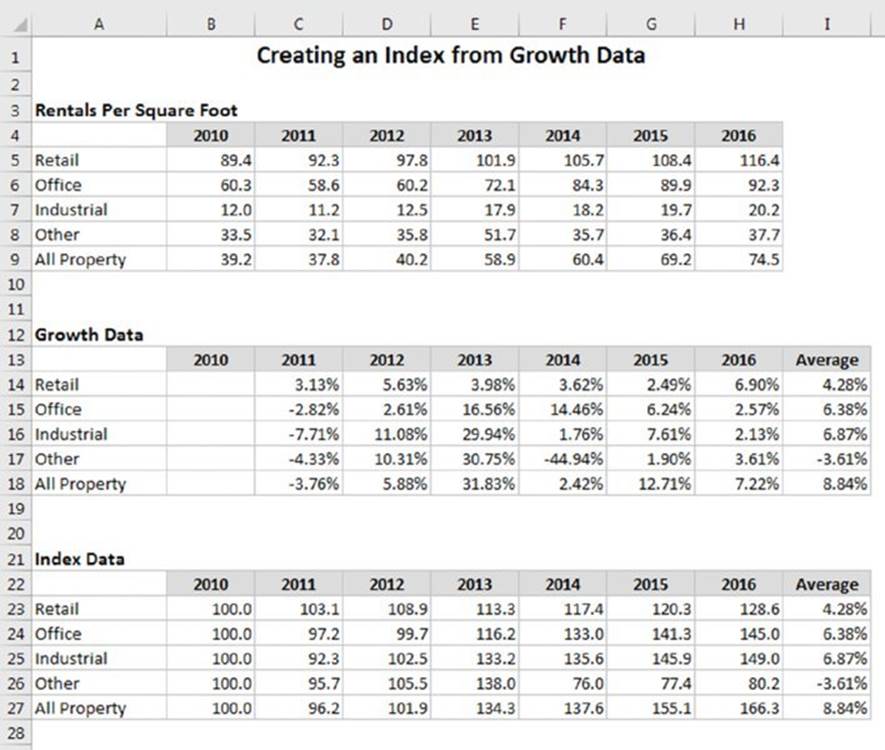
Figure 13.14 Creating an index from growth data.

On the Web

This example is available at this book’s website in the workbook indices.xlsx.

The formulas for calculating the growth rates (in the second table) are simple. For example, the formula in cell C14 follows:

=(C5–B5)/B5

This formula returns 3.13%, which represents the change in retail space (from $89.4 to $92.3). This formula is copied to the other cells in the table (range C14:H18). This information is useful, but it is difficult to track overall performance between periods of more than a year. That’s why indices are required.

Calculating the indices in the third table is also straightforward. The 2010 index is set at 100 (column B) and is the base for the indices. The formula in cell C23 follows:

=B23*(1+C14)

This formula is copied to the other cells in the table (range C23:H27).

These indices make it possible to compare performance of, say, offices between any two years and to track the relative performance over any two years of any two types of property. So it is clear, for example, that industrial property rental grew faster than retail property rentals between 2013 and 2016.

The average figures (column I) are calculated by using the RATE function. This results in an annual growth rate over the entire period.

Here’s the formula in cell I23 that calculates the average growth rate over the term:

=RATE(6,0,B23,–H23,0)

The nper argument is 6 in the formula because that is the number of years since the base date.