Excel 2016 Formulas (2016)

PART IV
Array Formulas

Chapter 15
Performing Magic with Array Formulas

In This Chapter

· More examples of single-cell array formulas

· More examples of multicell array formulas

The previous chapter introduced arrays and array formulas and presented some basic examples to whet your appetite. This chapter continues the saga and provides many useful examples that further demonstrate the power of this feature.

We selected the examples in this chapter to provide a good assortment of the various uses for array formulas. Most can be used as is. You do, of course, need to adjust the range names or references that you use. Also, you can modify many of the examples easily to work in a slightly different manner.

Working with Single-Cell Array Formulas

As we describe in the preceding chapter, you enter single-cell array formulas into a single cell (not into a range of cells). These array formulas work with arrays contained in a range or that exist in memory. This section provides some additional examples of such array formulas.

On the Web

The examples in this section are available at this book’s website. The file is named single-cell array formulas.xlsx.

About the examples in this chapter

This chapter contains many examples of array formulas. Keep in mind that you press Ctrl+Shift+Enter to enter an array formula. Excel places curly brackets around the formula to remind you that it’s an array formula. The array formula examples shown here are surrounded by curly brackets, but you should not enter the brackets because Excel does that for you when the formula is entered.

Summing a range that contains errors

You may have discovered that the SUM function doesn’t work if you attempt to sum a range that contains one or more error values (such as #DIV/0! or #N/A). Figure 15.1 shows an example. The formula in cell D11 returns an error value because the range that it sums (D4:D10) contains errors.

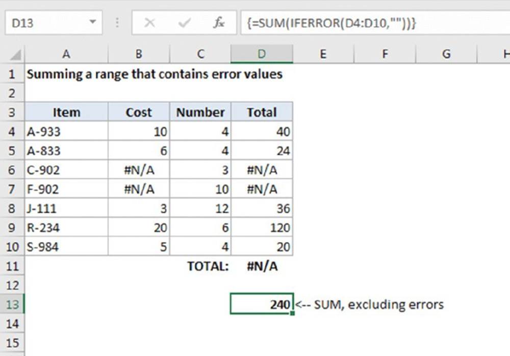
Figure 15.1 An array formula can sum a range of values, even if the range contains errors.

The following array formula, in cell D13, overcomes this problem and returns the sum of the values, even if the range contains error values:

{=SUM(IFERROR(D4:D10,""))}

This formula works by creating a new array that contains the original values but without the errors. The IFERROR function effectively filters out error values by replacing them with an empty string. The SUM function then works on this “filtered” array. This technique also works with other functions, such as AVERAGE, MIN, and MAX.

Note

The IFERROR function was introduced in Excel 2007. Following is a modified version of the formula that’s compatible with older versions of Excel:

{=SUM(IF(ISERROR(D4:D10),"",D4:D10))}

The AGGREGATE function, which works only in Excel 2010 and later, provides another way to sum a range that contains one or more error values. Here’s an example:

=AGGREGATE(9,2,D4:D10)

The first argument, 9, is the code for SUM. The second argument, 2, is the code for “ignore error values.”

Counting the number of error values in a range

The following array formula is similar to the previous example, but it returns a count of the number of error values in a range named Data:

{=SUM(IF(ISERROR(Data),1,0))}

This formula creates an array that consists of 1s (if the corresponding cell contains an error) and 0s (if the corresponding cell does not contain an error value).

You can simplify the formula a bit by removing the third argument for the IF function. If this argument isn’t specified, the IF function returns FALSE if the condition is not satisfied (that is, the cell does not contain an error value). In this context, Excel treats FALSE as a 0 value. The array formula shown here performs exactly like the previous formula, but it doesn’t use the third argument for the IF function:

{=SUM(IF(ISERROR(Data),1))}

Actually, you can simplify the formula even more:

{=SUM(ISERROR(Data)*1)}

This version of the formula relies on the fact that

TRUE * 1 = 1

and

FALSE * 1 = 0

Summing the n largest values in a range

The following array formula returns the sum of the ten largest values in a range named Data:

{=SUM(LARGE(Data,ROW(INDIRECT("1:10"))))}

The LARGE function is evaluated ten times, each time with a different second argument (1, 2, 3, and so on up to 10). The results of these calculations are stored in a new array, and that array is used as the argument for the SUM function.

To sum a different number of values, replace the 10 in the argument for the INDIRECT function with another value.

If the number of cells to sum is contained in cell C17, use the following array formula, which uses the concatenation operator (&) to create the range address for the INDIRECT function:

{=SUM(LARGE(Data,ROW(INDIRECT("1:"&C17))))}

To sum the n smallest values in a range, use the SMALL function instead of the LARGE function.

Computing an average that excludes zeros

Figure 15.2 shows a simple worksheet that calculates average sales. The formula in cell C13 follows:

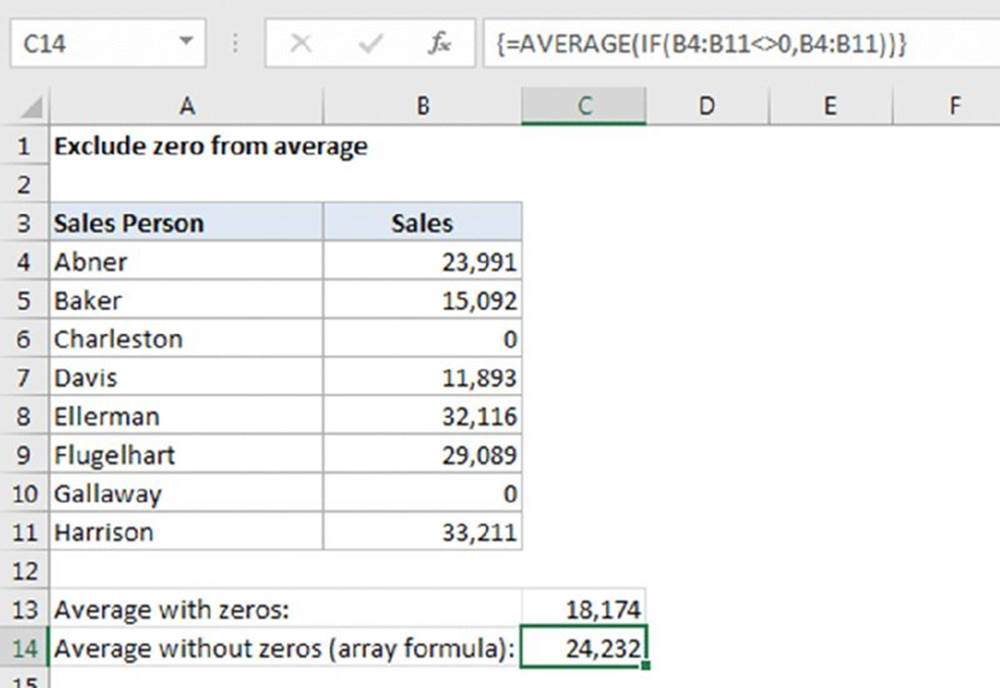
Figure 15.2 The calculated average includes cells that contain a 0.

=AVERAGE(B4:B11)

Two of the sales staff had the week off, however, so including their 0 sales in the calculated average doesn’t accurately describe the average sales per representative.

Note

The AVERAGE function ignores blank cells, but it does not ignore cells that contain 0.

The following array formula (in cell C14) returns the average of the range but excludes the cells containing 0:

{=AVERAGE(IF(B4:B11<>0,B4:B11))}

This formula creates a new array that consists only of the nonzero values in the range and FALSE in place of zero values. Many aggregate functions, including AVERAGE, ignore Boolean values just like they ignore blanks and text. The AVERAGE function then uses this new array as its argument.

You also can get the same result with a regular (nonarray) formula:

=SUM(B4:B11)/COUNTIF(B4:B11,"<>0")

This formula uses the COUNTIF function to count the number of nonzero values in the range. This value is divided into the sum of the values. This formula does not work if the range contains blank cells.

Note

The only reason to use an array formula to calculate an average that excludes zero values is for compatibility with versions prior to Excel 2007. A simple approach is to use the AVERAGEIF function in a nonarray formula:

=AVERAGEIF(B4:B11,"<>0",B4:B11)

Determining whether a particular value appears in a range

To determine whether a particular value appears in a range of cells, you can press Ctrl+F and do a search of the worksheet—or, you can make this determination by using an array formula.

Figure 15.3 shows a worksheet with a list of names in A5:E24 (named NameList). An array formula in cell D3 checks the name entered into cell C3 (named TheName). If the name exists in the list of names, the formula then displays the text Found. Otherwise, it displays Not Found.

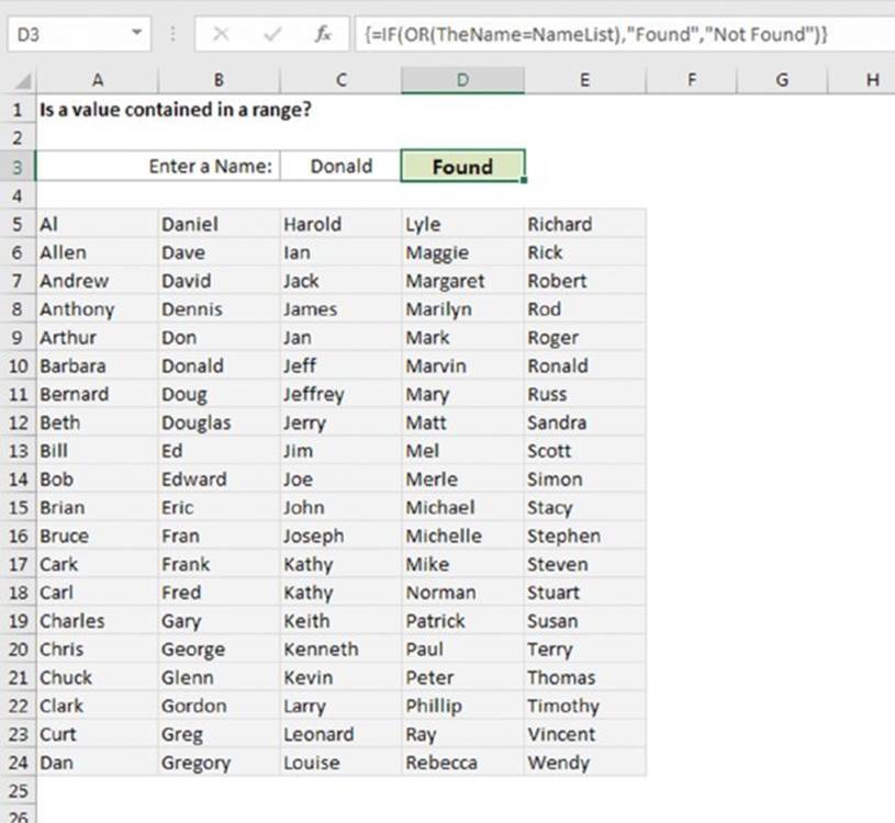
Figure 15.3 Using an array formula to determine whether a range contains a particular value.

The array formula in cell D3 is

{=IF(OR(TheName=NameList),"Found","Not Found")}

This formula compares TheName to each cell in the NameList range. It builds a new array that consists of logical TRUE or FALSE values. The OR function returns TRUE if any one of the values in the new array is TRUE. The IF function uses this result to determine which message to display.

A simpler form of this formula follows. This formula displays TRUE if the name is found and returns FALSE otherwise:

{=OR(TheName=NameList)}

Yet another approach uses the COUNTIF function in a nonarray formula:

=IF(COUNTIF(NameList,TheName)>0,"Found","Not Found")

Counting the number of differences in two ranges

The following array formula compares the corresponding values in two ranges (named MyData and YourData) and returns the number of differences in the two ranges. If the contents of the two ranges are identical, the formula returns 0.

{=SUM(IF(MyData=YourData,0,1))}

Figure 15.4 shows an example.

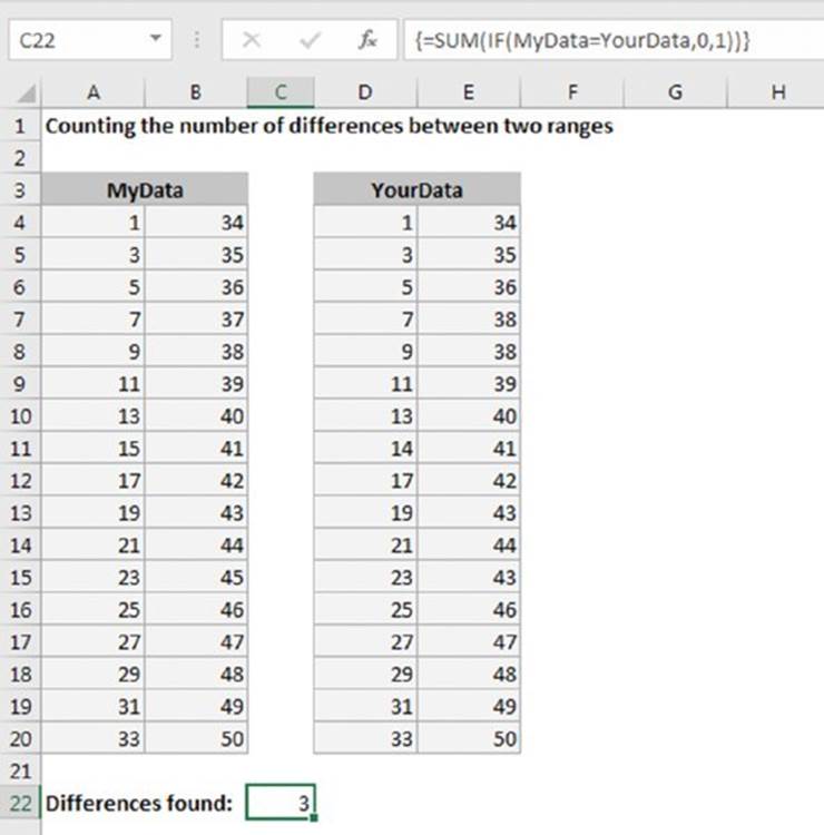
Figure 15.4 Using an array formula to count the number of differences in two ranges.

Note

The two ranges must be the same size and of the same dimensions.

This formula works by creating a new array of the same size as the ranges being compared. The IF function fills this new array with 0s and 1s (0 if a difference is found, and 1 if the corresponding cells are the same). The SUM function then returns the sum of the values in the array.

The following array formula, which is simpler, is another way of calculating the same result:

{=SUM(1*(MyData<>YourData))}

This version of the formula relies on the fact that

TRUE * 1 = 1

and

FALSE * 1 = 0

Once you know that comparisons return TRUE or FALSE and that Excel converts those to 1 and 0, respectively, you can manipulate the data in different ways to get the result you want. In yet another version of this formula, 1 is subtracted from each TRUE andFALSE, turning TRUE values into 0 and FALSE values into –1. Then the ABS function switches the sign:

{=ABS(SUM((MyData=YourData)-1))}

Returning the location of the maximum value in a range

The following array formula returns the row number of the maximum value in a single-column range named Data:

{=MIN(IF(Data=MAX(Data),ROW(Data), ""))}

The IF function creates a new array that corresponds to the Data range. If the corresponding cell contains the maximum value in Data, the array contains the row number; otherwise, it contains an empty string. The MIN function uses this new array as its second argument, and it returns the smallest value, which corresponds to the row number of the maximum value in Data.

If the Data range contains more than one cell that has the maximum value, the row of the first maximum cell is returned.

The following array formula is similar to the previous one, but it returns the actual cell address of the maximum value in the Data range. It uses the ADDRESS function, which takes two arguments: a row number and a column number.

{=ADDRESS(MIN(IF(Data=MAX(Data),ROW(Data), "")),COLUMN(Data))}

The previous formulas work only with a single-column range. The following variation works with any sized range and returns the address of the largest value in the range named Data:

{=ADDRESS(MIN(IF(Data=MAX(data),ROW(Data), "")),MIN(IF(Data=MAX(Data),COLUMN(Data), "")))}

Finding the row of a value’s nth occurrence in a range

The following array formula returns the row number within a single-column range named Data that contains the nth occurrence of the value in a cell named Value:

{=SMALL(IF(Data=Value,ROW(Data), ""),n)}

The IF function creates a new array that consists of the row number of values from the Data range that are equal to Value. Values from the Data range that aren’t equal to Value are replaced with an empty string. The SMALL function works on this new array and returns the nth smallest row number.

The formula returns #NUM! if the value is not found or if n exceeds the number of occurrences of the value in the range.

Returning the longest text in a range

The following array formula displays the text string in a range (named Data) that has the most characters. If multiple cells contain the longest text string, the first cell is returned:

{=INDEX(Data,MATCH(MAX(LEN(Data)),LEN(Data),FALSE),1)}

This formula works with two arrays, both of which contain the length of each item in the Data range. The MAX function determines the largest value, which corresponds to the longest text item. The MATCH function calculates the offset of the cell that contains the maximum length. The INDEX function returns the contents of the cell containing the most characters. This function works only if the Data range consists of a single column.

Figure 15.5 shows an example.

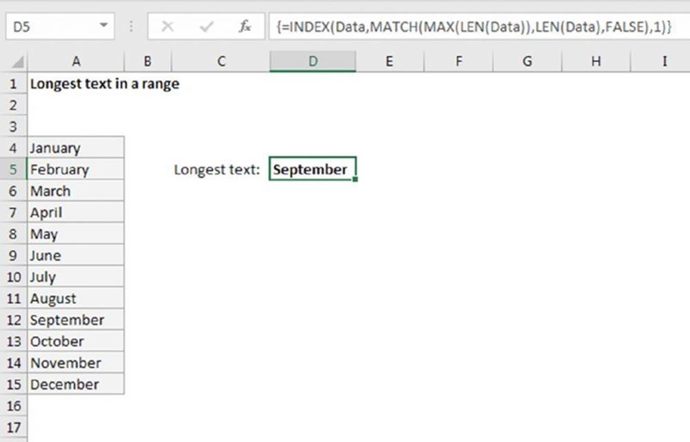
Figure 15.5 Using an array formula to return the longest text in a range.

Determining whether a range contains valid values

You may have a list of items that you need to check against another list. For example, you may import a list of part numbers into a range named MyList, and you want to ensure that all the part numbers are valid. You can do so by comparing the items in the imported list to the items in a master list of part numbers (named Master). Figure 15.6 shows an example.

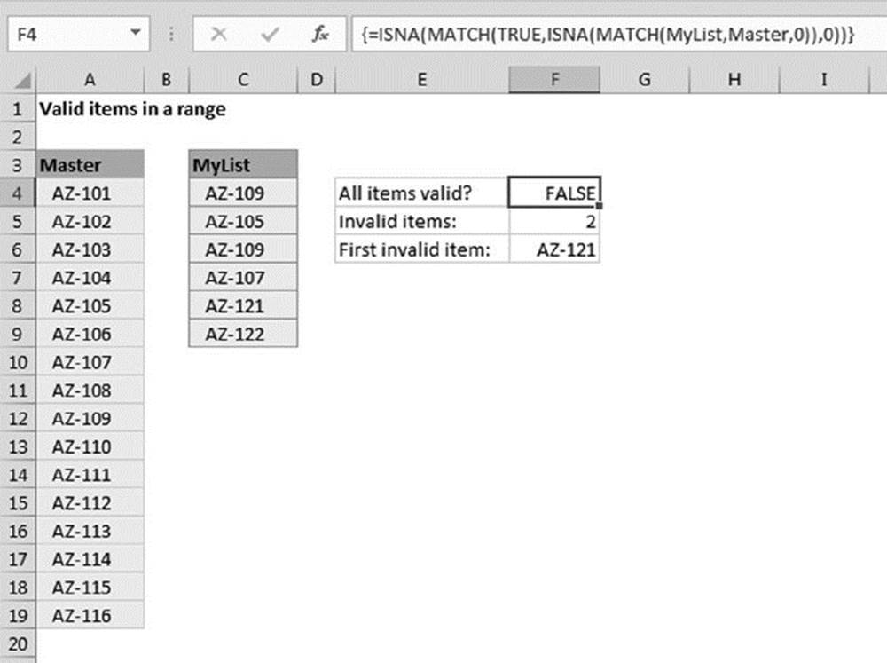
Figure 15.6 Using an array formula to count and identify items that aren’t in a list.

The following array formula returns TRUE if every item in the range named MyList is found in the range named Master. Both ranges must consist of a single column, but they don’t need to contain the same number of rows:

{=ISNA(MATCH(TRUE,ISNA(MATCH(MyList,Master,0)),0))}

The array formula that follows returns the number of invalid items. In other words, it returns the number of items in MyList that do not appear in Master:

{=SUM(1*ISNA(MATCH(MyList,Master,0)))}

To return the first invalid item in MyList, use the following array formula:

{=INDEX(MyList,MATCH(TRUE,ISNA(MATCH(MyList,Master,0)),0))}

Summing the digits of an integer

We can’t think of any practical application for the example in this section, but it’s a good demonstration of the potential power of an array formula. The following array formula calculates the sum of the digits in a positive integer, which is stored in cell A1. For example, if cell A1 contains the value 409, the formula returns 13 (the sum of 4, 0, and 9).

{=SUM(MID(A1,ROW(INDIRECT("1:"&LEN(A1))),1)*1)}

To understand how this formula works, start with the ROW function, as shown here:

{=ROW(INDIRECT("1:"&LEN(A1)))}

This function returns an array of consecutive integers beginning with 1 and ending with the number of digits in the value in cell A1. For example, if cell A1 contains the value 409, the LEN function returns 3, and the array generated by the ROW functions is

{1,2,3}

Cross-Ref

For more information about using the INDIRECT function to return this array, see Chapter 14, “Introducing Arrays.”

This array is then used as the second argument for the MID function. The MID part of the formula, simplified a bit and expressed as values, is the following:

{=MID(409,{1,2,3},1)*1}

This function generates an array with three elements:

{4,0,9}

By simplifying again and adding the SUM function, the formula looks like this:

{=SUM({4,0,9})}

This formula produces the result of 13.

Note

The values in the array created by the MID function are multiplied by 1 because the MID function returns a string. Multiplying by 1 forces a numeric value result. Alternatively, you can use the VALUE function to force a numeric string to become a numeric value.

Notice that the formula doesn’t work with a negative value because the negative sign is not a numeric value. Also, the formula fails if the cell contains nonnumeric values (such as 123A6). The following formula solves this problem by checking for errors in the array and replacing them with zero:

{=SUM(IFERROR(MID(A1,ROW(INDIRECT("1:"&LEN(A1))),1)*1,0))}

Note

This formula uses the IFERROR function, which was introduced in Excel 2007.

Figure 15.7 shows a worksheet that uses both versions of this formula.

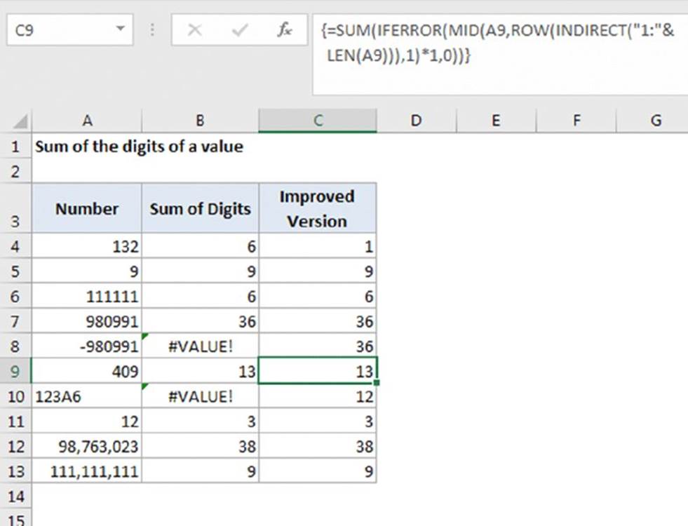
Figure 15.7 Two versions of an array formula that calculates the sum of the digits in an integer.

Summing rounded values

Figure 15.8 shows a simple worksheet that demonstrates a common spreadsheet problem: rounding errors. As you can see, the grand total in cell E7 appears to display an incorrect amount. (That is, it’s off by a penny.) The values in column E use a number format that displays two decimal places. The actual values, however, consist of additional decimal places that do not display due to rounding (as a result of the number format). The net effect of these rounding errors is a seemingly incorrect total. The total, which is actually $168.320997, displays as $168.32.

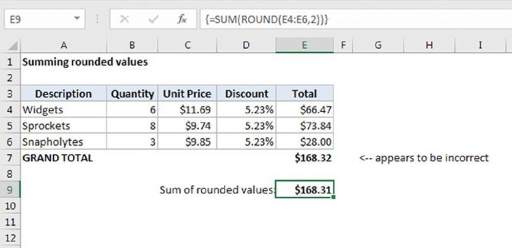
Figure 15.8 Using an array formula to correct rounding errors.

The following array formula creates a new array that consists of values in column E, rounded to two decimal places:

{=SUM(ROUND(E4:E6,2))}

This formula returns $168.31.

You also can eliminate these types of rounding errors by using the ROUND function in the formula that calculates each row total in column E (which does not require an array formula).

Summing every nth value in a range

Suppose that you have a range of values and you want to compute the sum of every third value in the list—the first, the fourth, the seventh, and so on. One solution is to hard-code the cell addresses in a formula. But a better solution is to use an array formula.

Note

In Figure 15.9, the values are stored in a range named Data, and the value of n is in cell D4 (named n).

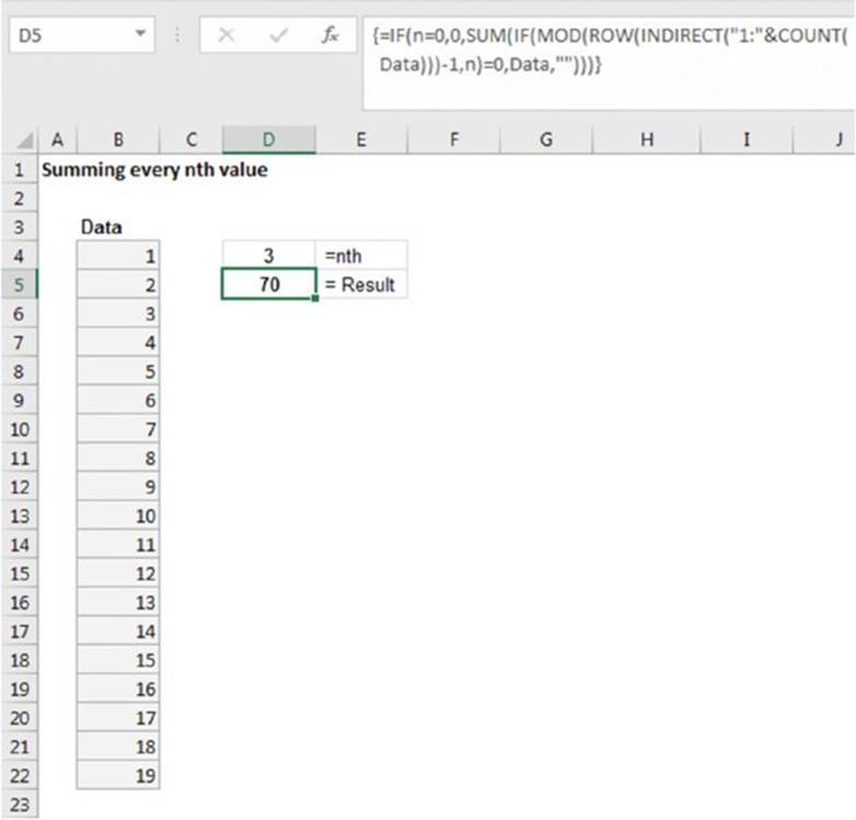
Figure 15.9 An array formula returns the sum of every nth value in the range.

The following array formula returns the sum of every nth value in the range:

{=SUM(IF(MOD(ROW(INDIRECT("1:"&COUNT(Data)))–1,n)=0,Data,""))}

This formula returns 70, which is the sum of every third value in the range.

This formula generates an array of consecutive integers, and the MOD function uses this array as its first argument. The second argument for the MOD function is the value of n. The MOD function creates another array that consists of the remainders when each row number minus 1 is divided by n. When the array item is 0 (that is, the row is evenly divisible by n), the corresponding item in the Data range is included in the sum.

You find that this formula fails when n is 0 (that is, when it sums no items). The modified array formula that follows uses an IF function to handle this case:

{=IF(n=0,0,SUM(IF(MOD(ROW(INDIRECT("1:"&COUNT(data)))–1,n)=0,data,"")))}

This formula works only when the Data range consists of a single column of values. It does not work for a multicolumn range or for a single row of values.

To make the formula work with a horizontal range, you need to transpose the array of integers generated by the ROW function. Excel’s TRANPOSE function is just the ticket. The modified array formula that follows works only with a horizontal Data range:

{=IF(n=0,0,SUM(IF(MOD(TRANSPOSE(ROW(INDIRECT("1:"&COUNT(Data))))–1,n)=0,Data,"")))}

Removing nonnumeric characters from a string

The following array formula extracts a number from a string that contains text. For example, consider the string ABC145Z. The formula returns the numeric part, 145.

{=MID(A1,MATCH(0,(ISERROR(MID(A1,ROW(INDIRECT("1:"&LEN(A1))),1)*1)*1),0),

LEN(A1)–SUM((ISERROR(MID(A1,ROW(INDIRECT("1:"&LEN(A1))),1)*1)*1)))}

This formula works only with a single embedded number. For example, it gives an incorrect result with a string like X45Z99 because the string contains two embedded numbers.

Using Excel’s Formula Evaluator

If you would like to better understand how some of these complex array formulas work, consider using a handy tool: the Formula Evaluator. Select the cell that contains the formula and then choose Formulas ➜ Formula Auditing ➜ Evaluate Formula. You’ll see the Evaluate Formula dialog box as shown in the figure.

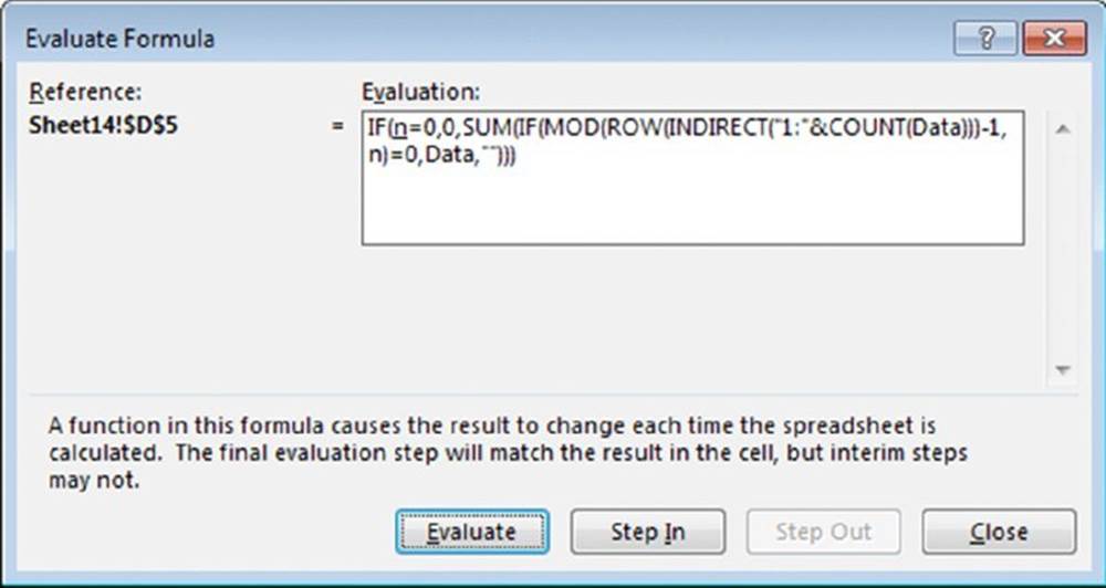
Click the Evaluate button repeatedly to see the intermediate results as the formula is being calculated. It’s like watching a formula calculate in slow motion.

Determining the closest value in a range

The formula in this section performs an operation that none of Excel’s lookup functions can do. The array formula that follows returns the value in a range named Data that is closest to another value (named Target):

{=INDEX(Data,MATCH(SMALL(ABS(Target-Data),1),ABS(Target-Data),0))}

If two values in the Data range are equidistant from the Target value, the formula returns the first one in the list. Figure 15.10 shows an example of this formula. In this case, the Target value is 45. The array formula in cell D4 returns 48—the value closest to 45.

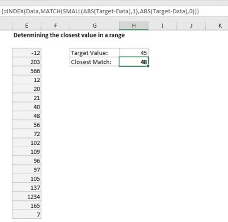
Figure 15.10 An array formula returns the closest match.

Returning the last value in a column

Suppose that you have a worksheet you update frequently by adding new data to columns. You may need a way to reference the last value in column A (the value most recently entered). If column A contains no empty cells, the solution is relatively simple and doesn’t require an array formula:

=OFFSET(A1,COUNTA(A:A)–1,0)

This formula uses the COUNTA function to count the number of nonempty cells in column A. This value (minus 1) is used as the second argument for the OFFSET function. For example, if the last value is in row 100, COUNTA returns 100. The OFFSET function returns the value in the cell 99 rows down from cell A1 in the same column.

If column A has one or more empty cells interspersed, which is frequently the case, the preceding formula doesn’t work because the COUNTA function doesn’t count the empty cells.

The following array formula returns the contents of the last nonempty cell in column A:

{=INDEX(A:A,MAX(ROW(A:A)*(NOT(ISBLANK(A:A)))))}

You can, of course, modify the formula to work with a column other than column A. To use a different column, change the column references from A to whatever column you need.

This formula does not work if the column contains error values.

Warning

You can’t use this formula, as written, in the same column in which it’s working. Attempting to do so generates a circular reference. You can, however, modify it. For example, to use the function in cell A1, change the references so that they begin with row 2 rather than the entire column. For example, use A2:A1000 to return the last nonempty cell in the range A2:A1000.

Tip

The formula that follows is an alternate (nonarray) formula that returns the last value in a column. This formula returns the last nonempty cell in column A:

=LOOKUP(2,1/(NOT(ISBLANK(A:A))),A:A )

The lookup_vector argument returns an array of 1 divided by either TRUE or FALSE, depending on whether the value in column A is blank. That evaluates down to an array of 1 for TRUE and a #DIV/0 error for FALSE. Finally, the LOOKUP function attempts to find a 2 in lookup_vector, ignoring errors along the way. When it gets to the end, not having found a 2, it returns the last value. It differs from the array formula in one way: it ignores error values. So it actually returns the last nonempty nonerror cell in a column.

Returning the last value in a row

The following array formula is similar to the previous formula, but it returns the last nonempty cell in a row (in this case, row 1):

{=INDEX(1:1,MAX(COLUMN(1:1)*(NOT(ISBLANK(1:1)))))}

To use this formula for a different row, change the 1:1 reference to correspond to the row.

Figure 15.11 shows an example for the last value in a column and the last value in a row.

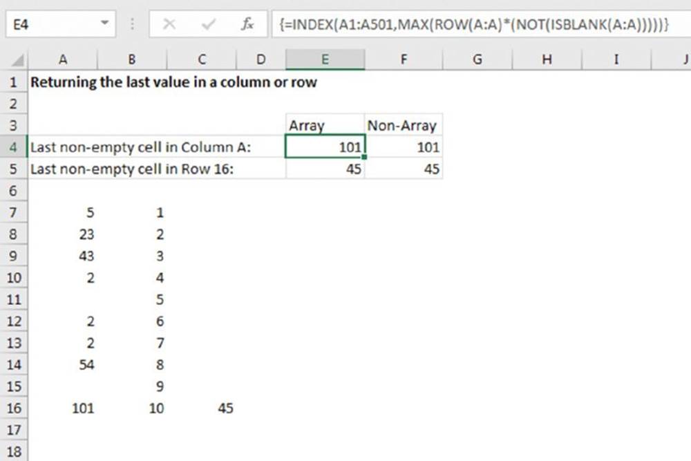
Figure 15.11 Using array formulas to return the last nonempty cell in a column or row.

An alternative, non-array formula that returns the last nonempty non-error cell in a row is

=LOOKUP(2,1/(NOT(ISBLANK(1:1))),1:1 )

Working with Multicell Array Formulas

The preceding chapter introduces array formulas that you can enter into multicell ranges. In this section, we present a few more multicell array formulas. Most of these formulas return some or all of the values in a range but are rearranged in some way.

When you enter a multicell array formula, you must select the entire range first. Then type the formula and press Ctrl+Shift+Enter.

On the Web

The examples in this section are available at this book’s website. The file is named multi-cell array formulas.xlsx.

Returning only positive values from a range

The following array formula works with a single-column vertical range (named Data). The array formula is entered into a range that’s the same size as Data and returns only the positive values in the Data range. (Zeroes and negative numbers are ignored.)

{=INDEX(Data,SMALL(IF(Data>0,ROW(INDIRECT("1:"&ROWS(Data)))),

ROW(INDIRECT("1:"&ROWS(Data)))))}

As you can see in Figure 15.12, this formula works, but not perfectly. The Data range is A4:A23, and the array formula is entered into C4:C23. However, the array formula displays #NUM! error values for cells that don’t contain a value.

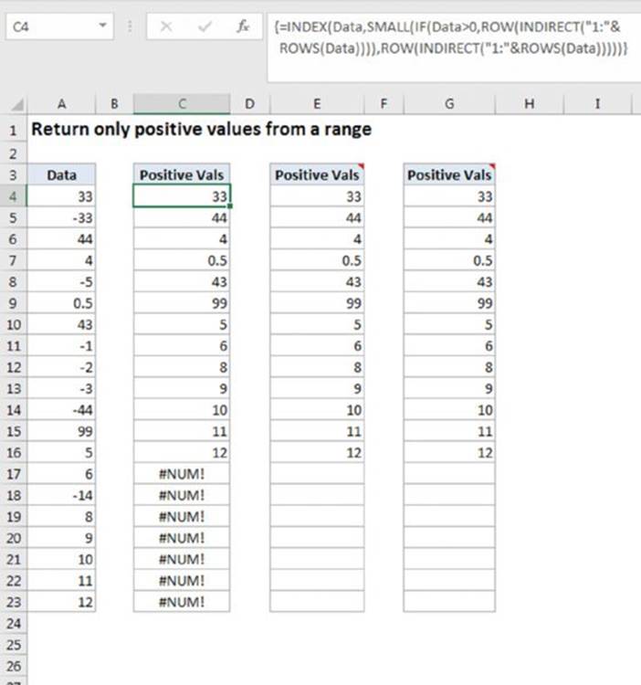
Figure 15.12 Using an array formula to return only the positive values in a range.

This modified array formula, entered into range E4:E23, uses the IFERROR function to avoid the error value display:

{=IFERROR(INDEX(Data,SMALL(IF(Data>0,ROW(INDIRECT("1:"&ROWS(Data)))),

ROW(INDIRECT("1:"&ROWS(Data))))),"")}

The IFERROR function was introduced in Excel 2007. For compatibility with older versions, use this formula entered in G4:G23:

{=IF(ISERR(SMALL(IF(Data>0,ROW(INDIRECT("1:"&ROWS(Data)))),

ROW(INDIRECT("1:"&ROWS(Data))))),"",INDEX(Data,SMALL(IF

(Data>0,ROW(INDIRECT("1:"&ROWS(Data)))),ROW(INDIRECT

("1:"&ROWS(Data))))))}

Returning nonblank cells from a range

The following formula is a variation on the formula in the preceding section. This array formula works with a single-column vertical range named Data. The array formula is entered into a range of the same size as Data and returns only the nonblank cell in the Datarange:

{=IFERROR(INDEX(Data,SMALL(IF(Data<>"",ROW(INDIRECT("1:"&ROWS(Data)))),

ROW(INDIRECT("1:"&ROWS(Data))))),"")}

For compatibility with versions prior to Excel 2007, use this formula:

{=IF(ISERR(SMALL(IF(Data<>"",ROW(INDIRECT("1:"&ROWS(Data)))),

ROW(INDIRECT("1:"&ROWS(Data))))),"",INDEX(Data,SMALL(IF(Data

<>"",ROW(INDIRECT("1:"&ROWS(Data)))),ROW(INDIRECT("1:"&ROWS

(Data))))))}

Reversing the order of cells in a range

In Figure 15.13, cells C4:C13 contain a multicell array formula that reverses the order of the values in the range A4:A13 (which is named Data).

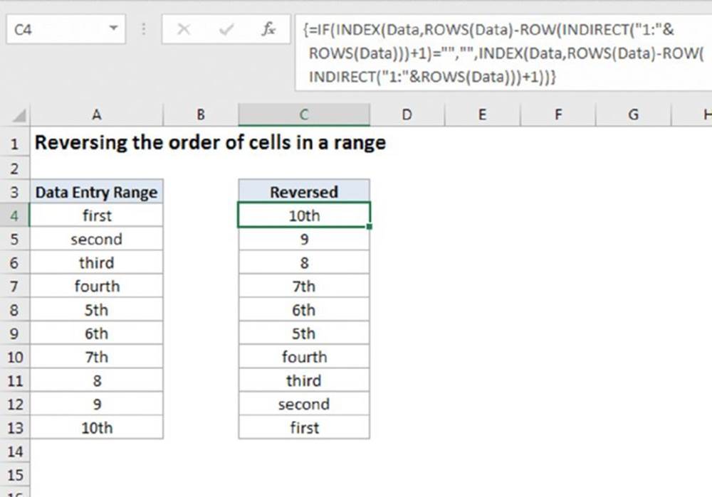
Figure 15.13 A multicell array formula displays the entries in A4:A13 in reverse order.

The array formula is

{=IF(INDEX(Data,ROWS(Data)-ROW(INDIRECT

("1:"&ROWS(Data)))+1)="","",INDEX(Data,ROWS(Data)–

ROW(INDIRECT("1:"&ROWS(Data)))+1))}

To reverse the order, a consecutive integer is subtracted from the total number of rows in the data. On its first iteration through the array, the first consecutive integer (1) is subtracted from the total rows (10) and 1 is added back to return 10. This is used in INDEX to retrieve the 10th cell in the range. The formula returns zero for blank cells, so an IF statement corrects that situation.

Sorting a range of values dynamically

Figure 15.14 shows a data entry range in column A (named Data). As the user enters values into that range, the values are displayed sorted from largest to smallest in column C. The array formula in column C is rather simple:

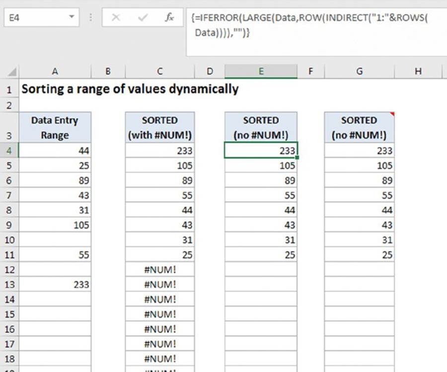
Figure 15.14 A multicell array formula displays the values in column A, sorted.

{=LARGE(Data,ROW(INDIRECT("1:"&ROWS(Data))))}

If you prefer to avoid the #NUM! error display, the formula gets a bit more complex:

{=IF(ISERR(LARGE(Data,ROW(INDIRECT("1:"&ROWS(Data))))),

"",LARGE(Data,ROW(INDIRECT("1:"&ROWS(Data)))))}

If you require compatibility with versions prior to Excel 2007, the formula gets even more complex:

{=IF(ISERR(LARGE(Data,ROW(INDIRECT("1:"&ROWS(Data))))),"",LARGE(Data,ROW(INDIRECT("1:"&ROWS(Data)))))}

Note that this formula works only with values. The file at this book’s website has a similar array formula example that works only with text.

Returning a list of unique items in a range

If you have a single-column range named Data, the following array formula returns a list of the unique items in the range (the list with no duplicated items):

{=INDEX(Data,SMALL(IF(MATCH(Data,Data,0)=ROW(INDIRECT

("1:"&ROWS(Data))),MATCH(Data,Data,0),""),ROW(INDIRECT

("1:"&ROWS(Data)))))}

This formula doesn’t work if the Data range contains blank cells. The unfilled cells of the array formula display #NUM!.

The following modified version eliminates the #NUM! display by using the IFERROR function, introduced in Excel 2007:

{=IFERROR(INDEX(Data,SMALL(IF(MATCH(Data,Data,0)=ROW(INDIRECT

("1:"&ROWS(data))),MATCH(Data,Data,0),""),ROW(INDIRECT

("1:"&ROWS(Data))))),"")}

Figure 15.15 shows an example. Range A4:A22 is named Data, and the array formula is entered into range C4:C22. Range E4:E23 contains the array formula that uses the IFERROR function.

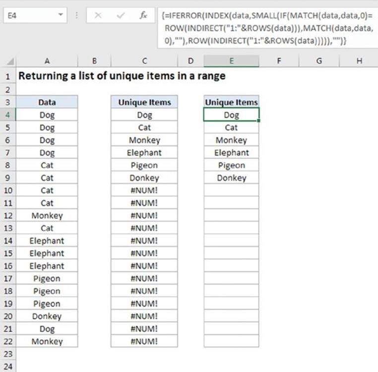
Figure 15.15 Using an array formula to return unique items from a list.

Displaying a calendar in a range

Figure 15.16 shows the results of one of our favorite multicell array formulas: a “live” calendar displayed in a range of cells. If you change the date at the top, the calendar recalculates to display the dates for the month and year.

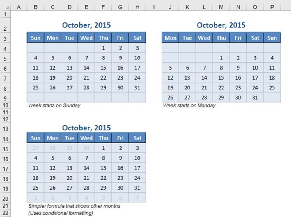
Figure 15.16 Displaying a calendar by using a single array formula.

On the Web

This workbook is available at this book’s website. The file is named array formula calendar.xlsx. In addition, the workbook contains an example that uses this technique to display a calendar for a complete year.

After you create this calendar, you can easily copy it to other worksheets or workbooks.

To create this calendar in the range B2:H9, follow these steps:

1. Select B2:H2 and merge the cells by choosing Home ➜ Alignment ➜ Merge & Center.

2. Type a date into the merged range.

The day of the month isn’t important.

3. Enter the abbreviated day names in the range B3:H3.

4. Select B4:H9 and enter this array formula.

Remember, to enter an array formula, use Ctrl+Shift+Enter (not just Enter).

{=IF(MONTH(DATE(YEAR(B2),MONTH(B2),1))<>MONTH(DATE(YEAR(B2),

MONTH(B2),1)-(WEEKDAY(DATE(YEAR(B2),MONTH(B2),1))–1)+

{0;1;2;3;4;5}*7+{1,2,3,4,5,6,7}–1),"",

DATE(YEAR(B2),MONTH(B2),1)–

(WEEKDAY(DATE(YEAR(B2),MONTH(B2),1))–1)+

{0;1;2;3;4;5}*7+{1,2,3,4,5,6,7}–1)}

5. Format the range B4:H9 to use this custom number format: d.

This step formats the dates to show only the day. Use the Custom category in the Number tab in the Format Cells dialog box to specify this custom number format.

6. Adjust the column widths and format the cells as you like.

Change the month and year in cell B2, and the calendar updates automatically. After creating this calendar, you can copy the range to any other worksheet or workbook.

The array formula actually returns date values, but the cells are formatted to display only the day portion of the date. Also, notice that the array formula uses array constants.

Cross-Ref

See Chapter 14 for more information about array constants.

The array formula can be simplified quite a bit by removing the IF function, which checks to make sure that the date is in the specified month:

=DATE(YEAR(B2),MONTH(B2),1)–(WEEKDAY(DATE(YEAR(B2),MONTH(B2),1))

–1)+{0;1;2;3;4;5}*7+{1,2,3,4,5,6,7}–1

This version of the formula displays the days from the preceding month and the next month.

Figure 15.17 shows 12 instances of the array formula calendar for an entire year.

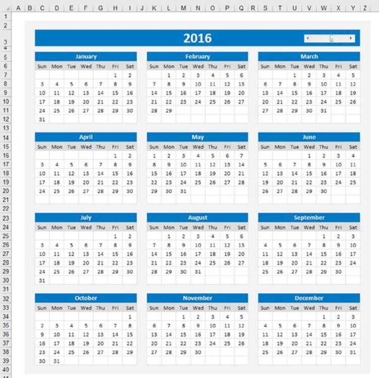
Figure 15.17 An annual calendar made from array formulas.