Excel 2016 Formulas (2016)

PART I
Understanding Formula Basics

Chapter 2
Basic Facts About Formulas

In This Chapter

· How to enter, edit, and paste names into formulas

· The various operators used in formulas

· How Excel calculates formulas

· Cell and range references used in formulas

· Copying and moving cells and ranges

· How to make an exact copy of a formula

· How to convert formulas to values

· How to prevent formulas from being viewed

· The types of formula errors

· Circular reference messages and correction techniques

· Excel’s goal seeking feature

This chapter serves as a basic introduction to using formulas in Excel. Although it’s intended primarily for newcomers to Excel, even veteran Excel users may find some new information here.

Entering and Editing Formulas

This section describes the basic elements of a formula. It also explains various ways of entering and editing your formulas.

Formula elements

A formula entered into a cell can consist of five elements:

§ Operators: These include symbols such as + (for addition) and * (for multiplication).

§ Cell references: These include named cells and ranges that can refer to cells in the current worksheet, cells in another worksheet in the same workbook, or even cells in a worksheet in another workbook.

§ Values or text strings: Examples include 7.5 (a value) and “Year-End Results” (a string, enclosed in quotes).

§ Worksheet functions and their arguments: These include functions such as SUM or AVERAGE and their arguments. Function arguments appear in parentheses and provide input for the function’s calculations.

§ Parentheses: These control the order in which expressions within a formula are evaluated.

Entering a formula

When you type an equal sign into an empty cell, Excel assumes that you are entering a formula because a formula always begins with an equal sign. Excel’s accommodating nature also permits you to begin your formula with a minus sign or a plus sign. However, Excel always inserts the leading equal sign after you enter the formula.

As a concession to former Lotus 1-2-3 users, Excel also allows you to use an “at” symbol (@) to begin a formula that starts with a function. For example, Excel accepts either of the following formulas:

=SUM(A1:A200)

@SUM(A1:A200)

However, after you enter the second formula, Excel replaces the @ symbol with an equal sign.

If your formula uses a cell reference, you can enter the cell reference in one of two ways: enter it manually, or enter it by pointing to cells that are used in the formula. We discuss each method in the following sections.

Entering a formula manually

Entering a formula manually involves, well, entering a formula manually. You simply activate a cell and type an equal sign (=) followed by the formula. As you type, the characters appear in the cell as well as in the Formula bar. You can, of course, use all the normal editing keys when typing a formula. After you insert the formula, press Enter.

Note

When you type an array formula, you must press Ctrl+Shift+Enter rather than just Enter. An array formula is a special type of formula, which we discuss in Part IV, “Array Formulas.”

After you press Enter, the cell displays the result of the formula. The formula itself appears in the Formula bar when the cell is activated.

Entering a formula by pointing

The other method of entering a formula that contains cell references still involves some manual typing, but you can simply point to the cell references instead of typing them manually. For example, to enter the formula =A1+A2 into cell A3, follow these steps:

1. Move the cell pointer to cell A3.

2. Type an equal sign (=) to begin the formula.

Notice that Excel displays Enter in the left side of the status bar.

3. Press the up arrow twice.

As you press this key, notice that Excel displays a moving border around the cell and that the cell reference (A1) appears in cell A3 and in the Formula bar. Also notice that Excel displays Point on the status bar.

If you prefer, you can use your mouse and click cell A1.

4. Type a plus sign (+).

The moving border becomes a solid blue border around A1, and Enter reappears in the status bar. The cell cursor also returns to the original cell (A3).

5. Press the up arrow one more time. If you prefer, you can use your mouse and click cell A2.

A2 is appended to the formula.

6. Press Enter to end the formula.

As with typing the formula manually, the cell displays the result of the formula, and the formula appears in the Formula bar when the cell is activated.

If you prefer, you can use your mouse and click the check mark icon next to the Formula bar instead of pressing Enter. And if, at any time, you change your mind about entering the formula, just press Esc or click the X icon next to the Formula bar.

This method might sound a bit tedious, but it’s actually very efficient after you get the hang of it. Pointing to cell addresses rather than entering them manually is almost always faster and more accurate.

Tip

Excel color-codes the range addresses and ranges when you are entering or editing a formula. This helps you quickly spot the cells that are used in a formula.

Cross-Ref

When you’re working with a table of data (created by using Insert ➜ Tables ➜ Table), you can use a different type of formula—a self-propagating formula that takes advantage of column names. We cover this topic in Chapter 9, “Working with Tables and Lists.”

Pasting names

As we discuss in Chapter 3, “Working with Names,” you can assign a name to a cell or range. If your formula uses named cells or ranges, you can type the name in place of the address or choose the name from a list and have Excel insert the name for you automatically.

To insert a name into a formula, position your cursor in the formula where you want the name entered and use one of these two methods:

§ Press F3 to display the Paste Name dialog box. Select the name and click OK.

§ Take advantage of the Formula AutoComplete feature. When you type a letter while constructing a formula, Excel displays a list of matching options. These options include functions and names.

Figure 2.1 shows Formula AutoComplete in use. In this case, SalesData is a defined range name. This name appears in the drop-down list, along with worksheet function names.

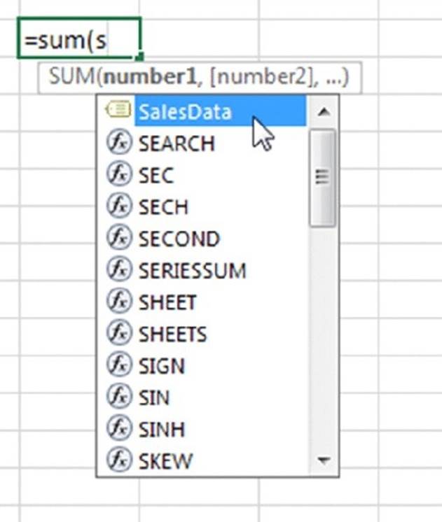
Figure 2.1 Using Formula AutoComplete to enter a range name into a formula.

Spaces and line breaks

Normally, you enter a formula without using spaces. However, you can use spaces (and even line breaks) within your formulas. Doing so has no effect on the formula’s result but can make the formula easier to read. To enter a line break in a formula, press Alt+Enter.Figure 2.2 shows a formula that contains spaces (indentions) and line breaks.

Figure 2.2 This formula contains spaces and line breaks.

Tip

To make the Formula bar display more than one line, drag the border below the Formula bar downward. Or click the downward-pointing icon at the extreme right of the Formula bar.

Formula limits

A formula can consist of up to about 8,000 characters. In the unlikely event that you need to create a formula that exceeds this limit, you must break the formula into multiple formulas. You also can opt to create a custom function by using Visual Basic for Applications (VBA).

Cross-Ref

Part VI, “Developing Custom Worksheet Functions,” focuses on creating custom functions.

Sample formulas

If you follow the preceding instructions for entering formulas, you can create a variety of them. This section looks at some sample formulas.

§ The following formula multiplies 150 × .01, returning 1.5. This formula uses only literal values, so it doesn’t seem very useful. However, it may be useful to show your work when you review your spreadsheet later:

=150*.01

§ This formula adds the values in cells A1 and A2:

=A1+A2

§ The next formula subtracts the value in the cell named Expenses from the value in the cell named Income:

=Income–Expenses

§ The following formula uses the SUM function to add the values in the range A1:A12:

=SUM(A1:A12)

§ The next formula compares cell A1 with cell C12 by using the = operator. If the values in the two cells are identical, the formula returns TRUE; otherwise, it returns FALSE:

=A1=C12

§ This final formula subtracts the value in cell B3 from the value in cell B2 and then multiplies the result by the value in cell B4:

=(B2–B3)*B4

Editing formulas

If you make changes to your worksheet, you may need to edit formulas. Or if a formula returns one of the error values described later in this chapter, you might need to edit the formula to correct the error. You can edit your formulas just as you edit any other cell.

Here are several ways to get into cell edit mode:

§ Double-click the cell. This enables you to edit the cell contents directly in the cell. This technique works only if the Double-click Allow Editing Directly in Cells check box is selected on the Advanced tab in the Excel Options dialog box.

§ Press F2. This enables you to edit the cell contents directly in the cell. If the Double-Click Allow Editing Directly in Cells check box is not selected, the editing occurs in the Formula bar.

§ Select the formula cell that you want to edit and then click in the Formula bar. This enables you to edit the cell contents in the Formula bar.

When you edit a formula, you can select multiple characters by dragging the mouse over them or by holding down Shift while you use the arrow keys. You can also press Home or End to select from the cursor position to the beginning or end of the current line of the formula.

Tip

Suppose you have a lengthy formula that contains an error, and Excel won’t let you enter it because of the error. In this case, you can convert the formula to text and tackle it again later. To convert a formula to text, just remove the initial equal sign (=). When you’re ready to return to editing the formula, insert the initial equal sign to convert the cell contents back to a formula.

Using the Formula bar as a calculator

If you simply need to perform a calculation, you can use the Formula bar as a calculator. For example, enter the following formula into any cell:

=(145*1.05)/12

Because this formula always returns the same result, you may prefer to store the formula’s result rather than the formula. To do so, press F2 to edit the cell. Then press F9, followed by Enter. Excel stores the formula’s result (12.6875) rather than the formula. This technique also works if the formula uses cell references.

This technique is most useful when you use worksheet functions. For example, to enter the square root of 221 into a cell, type =SQRT(221), press F9, and then press Enter. Excel enters the result: 14.8660687473185. You also can use this technique to evaluate just part of a formula. Consider this formula:

=(145*1.05)/A1

If you want to convert just the expression within the parentheses to a value, get into cell edit mode and select the part that you want to evaluate. In this example, select 145*1.05. Then press F9 followed by Enter. Excel converts the formula to the following:

=(152.25)/A1

Using Operators in Formulas

As previously discussed, an operator is one of the basic elements of a formula. An operator is a symbol that represents an operation. Table 2.1 shows the Excel-supported operators.

Table 2.1 Excel-Supported Operators

*Percent isn’t really an operator, but it functions similarly to one in Excel. Entering a percent sign after a number divides the number by 100. If the value is not part of a formula, Excel also formats the cell as percent.

Reference operators

Excel supports another class of operators known as reference operators; see Table 2.2. Reference operators work with cell references.

Table 2.2 Reference Operators

Sample formulas that use operators

These examples of formulas use various operators:

§ The following formula joins (concatenates) the two literal text strings (each enclosed in quotes) to produce a new text string: Part-23A:

="Part-"&"23A"

§ The next formula concatenates the contents of cell A1 with cell A2:

=A1&A2

§ Usually, concatenation is used with text, but concatenation works with values as well. For example, if cell A1 contains 123, and cell A2 contains 456, the preceding formula would return the value 123456. Note that, technically, the result is a text string. However, if you use this string in a mathematical formula, Excel treats it as a number. Some Excel functions ignore this “number” because they are designed to ignore text.

§ The following formula uses the exponentiation (^) operator to raise 6 to the third power to produce a result of 216:

=6^3

§ A more useful form of the preceding formula uses a cell reference instead of the literal value. Note this example that raises the value in cell A1 to the third power:

=A1^3

§ This formula returns the cube root of 216 (which is 6):

=216^(1/3)

§ The next formula returns TRUE if the value in cell A1 is less than the value in cell A2. Otherwise, it returns FALSE:

=A1<A2

§ Logical comparison operators also work with text. If A1 contains Alpha and A2 contains Gamma, the formula returns TRUE because Alpha comes before Gamma in alphabetical order.

§ The following formula returns TRUE if the value in cell A1 is less than or equal to the value in cell A2. Otherwise, it returns FALSE:

=A1<=A2

§ The next formula returns TRUE if the value in cell A1 does not equal the value in cell A2. Otherwise, it returns FALSE:

=A1<>A2

§ Excel doesn’t have logical AND and OR operators. Rather, you use functions to specify these types of logical operators. For example, this formula returns TRUE if cell A1 contains either 100 or 1000:

=OR(A1=100,A1=1000)

§ This last formula returns TRUE only if both cell A1 and cell A2 contain values less than 100:

=AND(A1<100,A2<100)

Operator precedence

You can (and should) use parentheses in your formulas to control the order in which the calculations occur. As an example, consider the following formula that uses references to named cells:

=Income–Expenses*TaxRate

The goal is to subtract expenses from income and then multiply the result by the tax rate. If you enter the preceding formula, though, you discover that Excel computes the wrong answer. The formula multiplies expenses by the tax rate and then subtracts the result from the income. In other words, Excel does not necessarily perform calculations from left to right (as you might expect).

The correct way to write this formula is

=(Income–Expenses)*TaxRate

To understand how this works, you need to be familiar with operator precedence—the set of rules that Excel uses to perform its calculations. Upcoming Table 2.3 lists Excel’s operator precedence. Operations are performed in the order listed in the table. For example, multiplication is performed before subtraction.

Table 2.3 Operator Precedence in Excel Formulas

Subtraction or negation?

One operator that can cause confusion is the minus sign (–), which you use for subtraction. However, a minus sign can also be a negation operator, which indicates a negative number.

Consider this formula:

=–3^2

Excel returns the value 9 (not –9). The minus sign serves as a negation operator and has a higher precedence than all other operators. The formula is evaluated as “negative 3, squared.” Using parentheses clarifies it:

=(–3)^2

The formula is not evaluated like this:

=–(3^2)

This is another example of why using parentheses, even if they are not necessary, is a good idea.

Use parentheses to override Excel’s built-in order of precedence. Returning to the previous example, the formula without parentheses is evaluated using Excel’s standard operator precedence. Because multiplication has a higher precedence, the Expenses cell multiplies by the TaxRate cell. Then this result is subtracted from Income—producing an incorrect calculation.

The correct formula uses parentheses to control the order of operations. Expressions within parentheses are always evaluated first. In this case, Expenses is subtracted from Income, and the result is multiplied by TaxRate.

Nested parentheses

You can also nest parentheses in formulas—that is, put parentheses inside parentheses. When a formula contains nested parentheses, Excel evaluates the most deeply nested expressions first and works its way out. The following example of a formula uses nested parentheses:

=((B2*C2)+(B3*C3)+(B4*C4))*B6

The preceding formula has four sets of parentheses. Three sets are nested inside the fourth set. Excel evaluates each nested set of parentheses and then sums the three results. This sum is then multiplied by the value in B6.

Make liberal use of parentheses in your formulas even when they aren’t necessary. Using parentheses clarifies the order of operations and makes the formula easier to read. For example, if you want to add 1 to the product of two cells, the following formula does the job:

=A1*A2+1

Because of Excel’s operator precedence rules, the multiplication will be performed before the addition. Therefore, parentheses are not necessary. You may find it much clearer, however, to use the following formula even though it contains superfluous parentheses:

=(A1*A2)+1

Tip

Every left parenthesis, of course, must have a matching right parenthesis. If you have many levels of nested parentheses, you may find it difficult to keep them straight. Fortunately, Excel lends a hand in helping you match parentheses. When editing a formula, matching parentheses are colored the same, although the colors can be difficult to distinguish if you have a lot of parentheses. Also, when the cursor moves over a parenthesis, Excel momentarily displays the parenthesis and its matching parenthesis in bold. This lasts for less than a second, so watch carefully.

Don’t hard-code values

When you create a formula, think twice before using a literal value in the formula. For example, if your formula calculates a 7.5 percent sales tax, you may be tempted to enter a formula such as this:

=A1*.075

A better approach is to insert the sales tax rate into a cell and use the cell reference in place of the literal value. This makes it easier to modify and maintain your worksheet. For example, if the sales tax range changes to 7.75 percent, you need to modify every formula that uses the old value. If the tax rate is stored in a cell, you simply change one cell, and all the formulas recalculate using the new value.

Calculating Formulas

You’ve probably noticed that the formulas in your worksheet are calculated immediately. If you change any cells that the formula uses, the formula displays a new result with no effort on your part. This occurs when Excel’s Calculation mode is set to Automatic. In this mode (the default mode), Excel follows certain rules when calculating your worksheet:

§ When you make a change (enter or edit data or formulas, for example), Excel calculates immediately those formulas that depend on new or edited data.

§ If working on a lengthy calculation, Excel temporarily suspends calculation when you need to perform other worksheet tasks; it resumes when you finish.

§ Formulas are evaluated in a natural sequence. For instance, if a formula in cell D12 depends on the result of a formula in cell F12, cell F12 is calculated before D12.

Sometimes, however, you may want to control when Excel calculates formulas. For example, if you create a worksheet with thousands of complex formulas, you may find that things can slow to a snail’s pace while Excel does its thing. In this case, you can set Excel’s Calculation mode to Manual. Do this by choosing Formulas ➜ Calculation➜ Calculation Options ➜ Manual.

When you work in manual Calculation mode, Excel displays Calculate in the status bar when you have any uncalculated formulas.

The Formulas ➜ Calculation group contains two controls that, when clicked, perform a calculation: Calculate Now and Calculate Sheet. In addition to these controls, you can click the Calculate word on the status bar or use the following shortcut keys to recalculate the formulas:

§ F9: Calculates the formulas in all open workbooks (same as the Calculate Now control).

§ Shift+F9: Calculates only the formulas in the active worksheet. It does not calculate other worksheets in the same workbook (same as the Calculate Sheet control).

§ Ctrl+Alt+F9: Forces a complete recalculation of all open workbooks. Use it if Excel (for some reason) doesn’t seem to return correct calculations.

§ Ctrl+Shift+Alt+F9: Rechecks all the dependent formulas and then forces a recalculation of all open workbooks.

Caution

Contrary to what you might expect, Excel’s Calculation mode isn’t specific to a particular workbook. When you change Excel’s Calculation mode, it affects all open workbooks—not just the active workbook. Also, the initial Calculation mode is set by the Calculation mode saved with the first workbook that you open.

Cell and Range References

Most formulas reference one or more cells by using the cell or range address (or the name if it has one). Cell references come in four styles; the use of the dollar sign symbol differentiates them:

§ Relative: The reference is fully relative. When you copy the formula, the cell reference adjusts to its new location.

Example: A1

§ Absolute: The reference is fully absolute. When you copy the formula, the cell reference does not change.

Example: $A$1

§ Row Absolute: The reference is partially absolute. When you copy the formula, the column part adjusts, but the row part does not change.

Example: A$1

§ Column Absolute: The reference is partially absolute. When you copy the formula, the row part adjusts, but the column part does not change.

Example: $A1

Creating an absolute or a mixed reference

When you create a formula by pointing to cells, all cell and range references are relative. To change a reference to an absolute reference or a mixed reference, you must do so manually by adding the dollar signs. Or when you’re entering a cell or range address, you can press the F4 key to cycle among all possible reference modes.

If you think about it, you may realize that the only reason you would ever need to change a reference is if you plan to copy the formula.

Figure 2.3 demonstrates an absolute reference in a formula. Cell D2 contains a formula that calculates a final sales price based on the quantity (cell B2), price (cell C2) and the sales tax (cell B7):

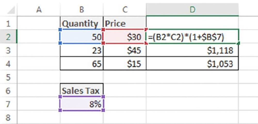
Figure 2.3 This worksheet demonstrates the use of an absolute reference.

=(B2*C2)*(1+$B$7)

The reference to cell B7 is an absolute reference. When you copy the formula in cell D2 to the cells below, the $B$7 reference always points to the sales tax cell. Using a relative reference (B7) results in incorrect results in the copied formulas.

Figure 2.4 demonstrates the use of mixed references. Note the formula in cell J3:

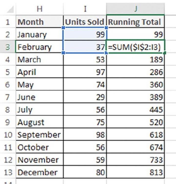
Figure 2.4 An example of using mixed references in a formula.

=SUM($I$2:I3)

This formula calculates a running total for Units Sold. Because the formula uses absolute references to row 2 and column I, each copied formula sums all Units Sold starting from cell I2. If the formula used relative references, copying the formula would cause that reference to adjust and produce the wrong results.

A1 versus R1C1 notation

Normally, Excel uses A1 notation. Each cell address consists of a column letter and a row number. However, Excel also supports R1C1 notation. In this system, cell A1 is referred to as cell R1C1, cell A2 as R2C1, and so on.

To change to R1C1 notation, choose File ➜ Options to open the Excel Options dialog box, click the Formulas tab, and place a check mark next to the R1C1 Reference Style option. Notice that all the column letters change to numbers. And all the cell and range references in your formulas adjust.

Look at the following examples of formulas using standard notation and R1C1 notation. The formula is assumed to be in cell B1 (also known as R1C2).

If you find R1C1 notation confusing, you’re not alone. R1C1 notation isn’t too bad when you’re dealing with absolute references. When relative references are involved, though, the brackets can drive you nuts.

The numbers in brackets refer to the relative position of the references. For example, R[–5]C[–3] specifies the cell that appears five rows above and three columns to the left. Conversely, R[5]C[3] references the cell that appears five rows below and three columns to the right. If you omit the brackets (or the numbers), it specifies the same row or column. For example, R[5]C refers to the cell five rows below in the same column.

Although you probably won’t use R1C1 notation as your standard system, it does have at least one good use. R1C1 notation makes it easy to spot an erroneous formula. When you copy a formula, every copied formula is the same in R1C1 notation. This remains true regardless of the types of cell references you use (relative, absolute, or mixed). Therefore, you can switch to R1C1 notation and check your copied formulas. If one looks different from its surrounding formulas, it’s probably incorrect.

However, you can take advantage of the background formula auditing feature, which can flag potentially incorrect formulas. We discuss this feature in Chapter 22, “Tools and Methods for Debugging Formulas.”

Referencing other sheets or workbooks

A formula can use references to cells and ranges that are in a different worksheet. To refer to a cell in a different worksheet, precede the cell reference with the sheet name followed by an exclamation point. Note this example of a formula that uses a cell reference in a different worksheet (Sheet2):

=Sheet2!A1+1

You can also create link formulas that refer to a cell in a different workbook. To do so, precede the cell reference with the workbook name (in square brackets), the worksheet name, and an exclamation point (!), like this:

=[Budget.xlsx]Sheet1!A1+1

If the workbook name or sheet name in the reference includes one or more spaces, you must enclose it (and the sheet name) in single quotation marks. For example:

='[Budget Analysis.xlsx]Sheet1'!A1+A1

If the linked workbook is closed, you must add the complete path to the workbook reference. For example:

='C:\MSOffice\Excel\[Budget Analysis.xlsx]Sheet1'!A1+A1

A linked file can also reside on another system that’s accessible on your corporate network. The following formula refers to a cell in a workbook in the files directory of a computer named DataServer:

='\\DataServer\files\[Budget Analysis.xlsx]Sheet1'!A1

If the linked workbook is stored on the Internet, the formula also includes the uniform resource locator (URL). For example:

='https://d.docs.live.net/86a61fd208/files/[Annual Budget.xlsx]Sheet1'!A1

Opening a workbook with external reference formulas

When you open a workbook that contains links, Excel displays a dialog box that asks whether you want to do the following:

· Update: The links are updated with the current information in the source file(s).

· Don’t Update: The links are not updated, and the workbook displays the previous values returned by the link formulas.

· Help: The Excel Help screen displays so you can read about links.

What if you choose to update the links, but the source workbook is no longer available? If Excel can’t locate a source workbook that’s referred to in a link formula, it displays its Edit Links dialog box. Click the Change Source button to specify a different workbook or click the Break Link to destroy the link.

Although you can enter link formulas directly, you can also create the reference by using the normal pointing methods discussed earlier. To do so, make sure the source file is open. Normally, you can create a formula by pointing to results in relative cell references. But when you create a reference to another workbook by pointing, Excel always creates absolute cell references. If you plan to copy the formula to other cells, you must edit the formula to make the references relative.

Caution

Working with links can be tricky and may cause some unexpected problems. For example, if you use the File ➜ Save As command to make a backup copy of the source workbook, you automatically change the link formulas to refer to the new file (not usually what you want). You can also mess up your links by renaming the source workbook file.

Copying or Moving Formulas

As you create a worksheet, you may find it necessary to copy or move information from one location to another. Excel makes copying or moving ranges of cells easy. Here are some common things you might do:

§ Copy a cell to another location. Contents of the source cell are duplicated in the destination cell.

§ Copy a cell to a range of cells. The source cell is copied to every cell in the destination range.

§ Copy a range to another range. Both ranges must be the same size.

§ Move a range of cells to another location. Contents are removed from the source cell and relocated to the destination.

The primary difference between copying and moving a range is the effect of the operation on the source range. When you copy a range, the source range is unaffected. When you move a range, the contents are removed from the source range.

Note

Copying a cell normally copies the cell’s contents, any formatting that is applied to the original cell (including conditional formatting and data validation), and the cell comment (if it has one). When you copy a cell that contains a formula, the cell references in the copied formulas are changed automatically to be relative to their new destination.

Copying or moving consists of two steps (although shortcut methods are available):

1. Select the cell or range to copy (the source range) and copy it to the Clipboard. To move the range instead of copying it, cut the range rather than copying it.

2. Move the cell pointer to the range that will hold the copy (the destination range), and paste the Clipboard contents.

Caution

When you paste information, Excel overwrites any cells that get in the way without warning you. If you find that pasting overwrote some essential cells, choose Undo from the Quick Access toolbar (or press Ctrl+Z).

Note

When you copy a cell or range, Excel surrounds the copied area with an animated border. As long as that border remains animated, the copied information is available for pasting. If you press Esc to cancel the animated border, Excel removes the information from the Clipboard.

When you copy a range that contains formulas, the cell references in the formulas are adjusted. When you move a range that contains formulas, the cell references in the formulas are not adjusted. This is almost always what you want.

About the Office Clipboard

Whenever you cut or copy information from a Windows program, Windows stores the information on the Windows Clipboard, which is an area of your computer’s memory. Each time that you cut or copy information, Windows replaces the information previously stored on the Clipboard with the new information that you cut or copied. The Windows Clipboard can store data in a variety of formats. Because Windows manages information on the Clipboard, it can be pasted to other Windows applications, regardless of where it originated.

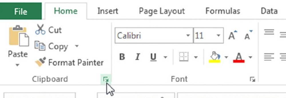
Microsoft Office has its own Clipboard (the Office Clipboard), which is available only in Office programs. To view or hide the Office Clipboard, click the dialog launcher icon in the bottom-right corner of the Home ➜ Clipboard group.

Whenever you cut or copy information in an Office program, such as Excel or Word, the program places the information on both the Windows Clipboard and the Office Clipboard. However, the program treats information on the Office Clipboard differently than it treats information on the Windows Clipboard. Instead of replacing information on the Office Clipboard, the program appends the information to the Office Clipboard. With multiple items stored on the Clipboard, you can then paste the items individually or as a group.

The Office Clipboard has a serious problem that makes it virtually worthless for Excel users: if you copy a range that contains formulas, the formulas are not transferred when you paste to a different range. Only the values are pasted. Furthermore, Excel doesn’t even warn you about this fact.

Making an Exact Copy of a Formula

When you copy a formula, Excel adjusts the formula’s cell references when you paste it to a different location. Usually, adjusting the cell references is exactly what you want. Sometimes, however, you may want to make an exact copy of the formula. You can do this by converting the cell references to absolute references, as discussed earlier—but this isn’t always desirable.

A better approach is to select the formula while in edit mode and then copy it to the Clipboard as text. There are several ways to do this. Here we present a step-by-step example of how to make an exact copy of the formula in A1 and copy it to A2:

1. Select cell A1 and press F2 to activate edit mode.

2. Press Ctrl+Home to move the cursor to the start of the formula, followed by Ctrl+Shift+End to select all the formula text.

Or you can drag the mouse to select the entire formula.

Note that holding down the Ctrl key is necessary when the formula is more than one line long, but it’s optional for formulas that are a single line.

3. Choose Home ➜ Clipboard ➜ Copy (or press Ctrl+C).

This copies the selected text to the Clipboard.

4. Press Esc to end edit mode.

5. Activate cell A2.

6. Press F2 for edit mode.

7. Choose Home ➜ Clipboard ➜ Paste (or press Ctrl+V), followed by Enter.

This operation pastes an exact copy of the formula text into cell A2.

You can also use this technique to copy just part of a formula to use in another formula. Just select the part of the formula that you want to copy by dragging the mouse or by pressing the Shift+arrow keys. Then use any of the available techniques to copy the selection to the Clipboard. After that, you can paste the text to another cell.

Formulas (or parts of formulas) copied in this manner won’t have their cell references adjusted when you paste them to a new cell. This is because you copy the formulas as text, not as actual formulas.

Another technique for making an exact copy of a formula is to edit the formula and remove its initial equal sign. This converts the formula to text. Then copy the “nonformula” to a new location. Finally, edit both the original formula and the copied formula by inserting the initial equal sign.

Converting Formulas to Values

If you have a range of formulas that always produce the same result (that is, dead formulas), you may want to convert them to values. You can use the Home ➜ Clipboard➜ Paste ➜ Values command to do this.

Suppose that range A1:A10 contains formulas that calculate results that never change. To convert these formulas to values, do the following:

1. Select A1:A10.

2. Choose Home ➜ Clipboard ➜ Copy (or press Ctrl+C).

3. Choose Home ➜ Clipboard ➜ Paste ➜ Values (V).

4. Press Enter or Esc to cancel paste mode.

You can also take advantage of a drop-down control that shows paste options. In step 3 in the preceding list, press Ctrl+V to paste. A drop-down list appears at the lower-right corner of the range. Click and select one of the Paste Values icons (see Figure 2.5).

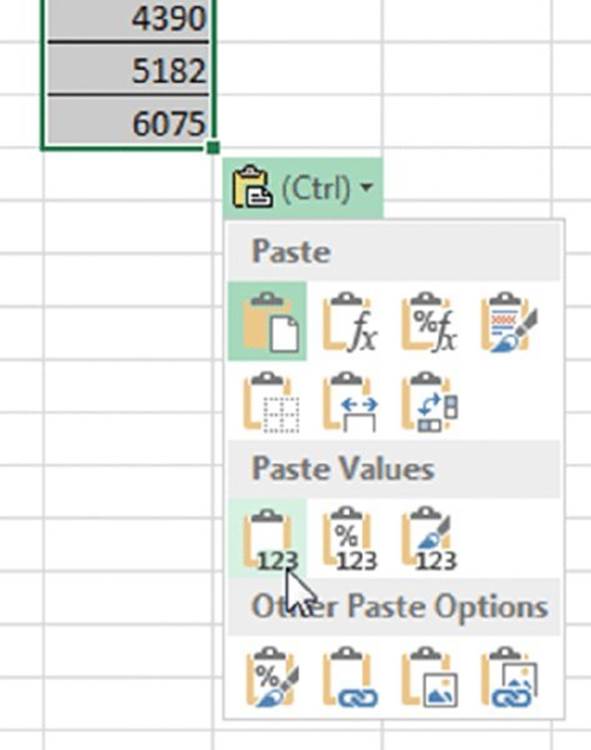
Figure 2.5 Choosing a paste option after pasting data.

Converting formulas to values is useful when you use formulas as a means to convert cells. For example, assume that you have a list of names (in uppercase) in column A. You want to convert these names to proper case. To do so, you need to create formulas in a separate column; then convert the formulas to values and replace the original values in column A. The following steps illustrate how to do this:

1. Insert a new column after column A.

2. Insert the following formula into cell B1:

=PROPER(A1)

3. Copy the formula down column B to accommodate the number of entries in column A.

Column B then displays the values in column A, but in proper case.

4. Select all the names in column B.

5. Choose Home ➜ Clipboard ➜ Copy.

6. Select cell A1.

7. Choose Home ➜ Clipboard ➜ Paste ➜ Values.

8. Press Enter or Esc to cancel paste mode.

9. Delete column B.

When to use AutoFill rather than formulas

Excel’s AutoFill feature provides a quick way to copy a cell to adjacent cells. AutoFill also has some other uses that may substitute for formulas in some cases. Many experienced Excel users don’t take advantage of the AutoFill feature, which can save a lot of time.

For example, if you need values from 1 to 100 to appear in A1:A100, you can do it with formulas. You type 1 into cell A1, type the formula =A1+1 into cell A2, and then copy the formula to the 98 cells below.

You can also use AutoFill to create the series for you without using a formula. To do so, type 1 into cell A1 and 2 into cell A2. Select A1:A2 and drag the fill handle down to cell A100. (The fill handle is the small square at the lower-right corner of the active cell.) When you use AutoFill in this manner, Excel analyzes the selected cells and uses this information to complete the series. If cell A1 contains 1 and cell A2 contains 3, Excel recognizes this pattern and fills in 5, 7, 9, and so on. This also works with decreasing series (10, 9, 8, and so on) and dates. If there is no discernible pattern in the selected cells, Excel performs a linear regression and fills in values on the calculated trend line.

Excel also recognizes common series names such as months and days of the week. If you type Monday into a cell and then drag its fill handle, Excel fills in the successive days of the week. You also can create custom AutoFill lists using the Custom Lists panel in the Excel Options dialog box. Finally, if you drag the fill handle with the right mouse button, Excel displays a shortcut menu to enable you to select an AutoFill option.

Tip

Flash Fill can be an alternative to formulas. See Chapter 16, “Importing and Cleaning Data,” for more information about Flash Fill.

Hiding Formulas

In some cases, you may not want others to see your formulas. For example, you may have a special formula you developed that performs a calculation proprietary to your company. You can use the Format Cells dialog box to hide the formulas contained in these cells.

To prevent one or more formulas from being viewed:

1. Select the formula or formulas.

2. Right-click and choose Format Cells to show the Format Cells dialog box (or press Ctrl+1).

3. In the Format Cells dialog box, click the Protection tab.

4. Place a check mark in the Hidden check box, as shown in Figure 2.6.

5. Use the Review ➜ Changes ➜ Protect command to protect the worksheet.

To prevent others from unprotecting the sheet, specify a password in the Protect Sheet dialog box.

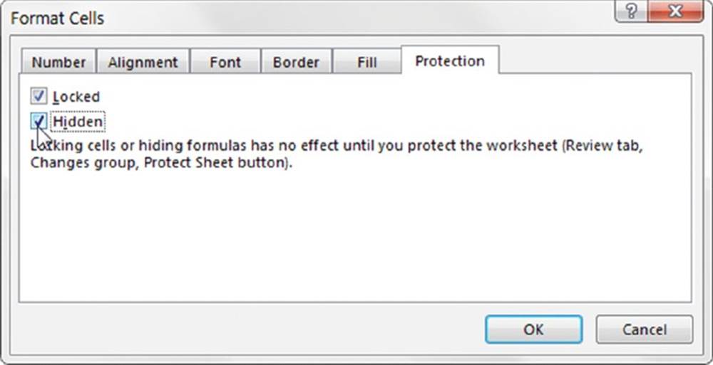
Figure 2.6 Use the Format Cells dialog box to change the Hidden and Locked status of a cell or range.

By default, all cells are locked. Protecting a sheet prevents any locked cells from being changed. So you should unlock any cells that require user input before protecting your sheet.

Caution

Be aware that it’s easy to crack the password for a worksheet. So this technique of hiding your formulas does not ensure that no one can view them.

Errors in Formulas

It’s not uncommon to enter a formula only to find that the formula returns an error. Table 2.4 lists the types of error values that may appear in a cell that has a formula.

Table 2.4 Excel Error Values

Note

Formulas may return an error value if a cell that they refer to has an error value. This is known as the ripple effect: a single error value can make its way to lots of other cells that contain formulas that depend on that cell.

If the entire cell fills with hash marks (#########), this usually means that the column isn’t wide enough to display the value. You can either widen the column or change the number format of the cell. The cell also fills with hash marks if it contains a formula that returns an invalid date or time.

Caution

Refer to Chapter 22 for more information about identifying and tracing errors.

Dealing with Circular References

When you enter formulas, you may occasionally see a message from Excel like the one shown in Figure 2.7. This indicates that the formula you just entered will result in a circular reference.

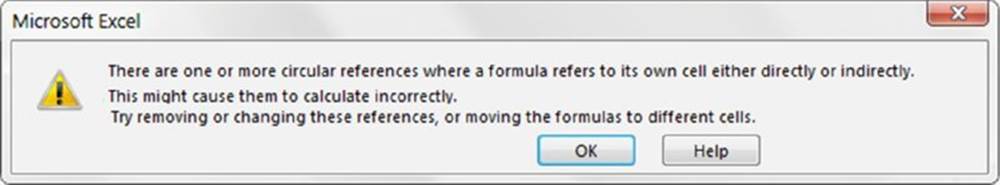
Figure 2.7 Excel’s way of telling you that your formula contains a circular reference.

A circular reference occurs when a formula refers to its own value, either directly or indirectly. For example, if you type =A1 into cell A3, =A3 into cell B3, and =B3 into cell A1, it produces a circular reference because the formulas create a circle in which each formula depends on the one before it. Every time the formula in A3 is calculated, it affects the formula in B3, which in turn affects the formula in A1. The result of the formula in A1 then causes A3 to recalculate, and the calculation circle starts all over again.

When you enter a formula that contains a circular reference, Excel displays a dialog box with two options: OK and Help.

Normally, you’ll want to correct any circular references, so you should click OK. After you do so, Excel inserts tracing arrows. Clicking the Help option displays the Excel Help topic for circular references.

The status bar displays Circular References: A3, in this case. To resolve the circular reference, choose Formulas ➜ Formula Auditing ➜ Error Checking ➜ Circular References to see a list of the cells involved in the circular reference. Click each cell in turn and try to locate the error. If you cannot determine whether the cell is the cause of the circular reference, navigate to the next cell on the Circular References submenu. Continue reviewing each cell on the Circular References submenu until the status bar no longer readsCircular References.

Tip

Instead of navigating to each cell using the Circular References submenu, you can click the tracer arrows to quickly jump between cells.

After you enter a formula that contains a circular reference, Excel displays a message in the status bar reminding you that a circular reference exists. In this case, the message reads Circular References: A3. If you activate a different worksheet or workbook, the message simply displays Circular References (without the cell reference).

Caution

Excel doesn’t warn you about a circular reference if you have the Enable Iterative Calculation setting turned on. You can check this in the Excel Options dialog box (in the Calculation section of the Formulas tab). If this option is checked, Excel performs the circular calculation the number of times specified in the Maximum Iterations field (or until the value changes by less than .001—or whatever other value appears in the Maximum Change field). You should, however, keep the Enable Iterative Calculation setting off so that you’ll be warned of circular references. Generally, a circular reference indicates an error that you must correct.

When the formula in a cell refers to that cell, the cause of the circular reference is quite obvious and is, therefore, easy to identify and correct. For this type of circular reference, Excel does not show tracer arrows. For an indirect circular reference, as in the preceding example, the tracer arrows can help you identify the problem.

Goal Seeking

Many spreadsheets contain formulas that enable you to ask questions such as, “What would be the total profit if sales increase by 20 percent?” If you set up your worksheet properly, you can change the value in one cell to see what happens to the profit cell.

Goal seeking serves as a useful feature that works in conjunction with your formulas. If you know what a formula result should be, Excel can tell you which values of one or more input cells you need to produce that result. In other words, you can ask a question such as, “What sales increase is needed to produce a profit of $1.2 million?”

Single–cell goal seeking (also known as backsolving) represents a rather simple concept. Excel determines what value in an input cell produces a desired result in a formula cell. You can best understand how this works by walking through an example.

A goal seeking example

Figure 2.8 shows a loan payment calculator that shows the expected monthly payment based on a given loan amount, number of payment months, and interest rate.

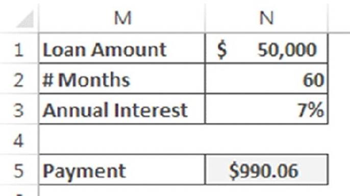
Figure 2.8 This worksheet presents a simple demonstration of goal seeking.

Imagine that you know you can afford a payment of $500 per month. Knowing you can get a fixed-rate of 7 percent over 60 payment months, what is the maximum loan you can take and still have a payment of $500?

In other words, what value in cell N1 causes the formula in cell N5 to yield $500? You can plug values into cell N1 until N5 displays $500. Or you can let Excel determine the answer.

To answer this question, choose Data ➜ Data Tools ➜ What-If Analysis ➜ Goal Seek. Excel displays the Goal Seek dialog box, as shown in Figure 2.9. Completing this dialog box resembles forming the following sentence: set cell N5 to 500 by changing cell N1. Clicking OK begins the goal seeking process.

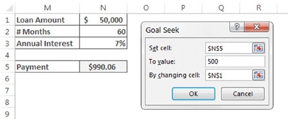
Figure 2.9 The Goal Seek dialog box.

Almost immediately, Excel announces that it has found the solution and displays the Goal Seek status box (see Figure 2.10). This box tells you the target value and what Excel came up with. In this case, Excel found that a loan amount of $25,251 would yield $500 monthly payments.

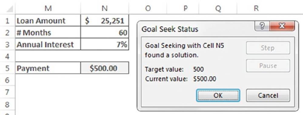
Figure 2.10 The Goal Seek Status dialog box.

You can click OK to replace the original value with the found value, or you can click Cancel to restore your worksheet to its original form before you chose Goal Seek.

More about goal seeking

If you think about it, you may realize that Excel can’t always find a value that produces the result you’re looking for—sometimes a solution doesn’t exist. In such a case, the Goal Seek Status box informs you of that fact. Other times, however, Excel may report that it can’t find a solution even though you believe one exists. In this case, you can adjust the current value of the changing cell to a value closer to the solution and then reissue the command. If that fails, double-check your logic and make sure that the formula cell does indeed depend on the specified changing cell.

Like all computer programs, Excel has limited precision. To demonstrate this, enter =A1^2 into cell A2. Then choose Data ➜ Data Tools ➜ What-If Analysis ➜ Goal Seek to find the value in cell A1 that causes the formula to return 16. Excel returns a value of 4.00002269—close to the square root of 16, but certainly not exact. You can adjust the precision in the Calculation section of the Formulas tab in the Excel Options dialog box (make the Maximum change value smaller).

In some cases, multiple values of the input cell produce the same desired result. For example, the formula =A1^2 returns 16 if cell A1 contains either –4 or +4. If you use goal seeking when two solutions exist, Excel gives you the solution that is nearest to the current value in the cell.

Perhaps the main limitation of the Goal Seek command is that it can find the value for only one input cell. For example, it can’t tell you what purchase price and what down payment percent result in a particular monthly payment. If you want to change more than one variable at a time, use the Solver add-in.