Excel 2016 Formulas (2016)
PART V
Miscellaneous Formula Techniques
Chapter 20
Using Data Validation
In This Chapter
· An overview of Excel’s data validation feature
· Practical examples of using data validation formulas
This chapter explores a useful Excel feature: data validation. Data validation enables you to add rules for what’s acceptable in specific cells and allows you to add dynamic elements to your worksheet without using macro programming.
About Data Validation
The Excel data validation feature allows you to set up rules that dictate what can be entered into a cell. For example, you may want to limit data entry in a particular cell to whole numbers between 1 and 12. You can specify an input message to help the user know what kind of data to enter in the cell. If the user makes an invalid entry, you can display a custom message. Figure 20.1 shows an example of both the input message and the message generated from an invalid entry.
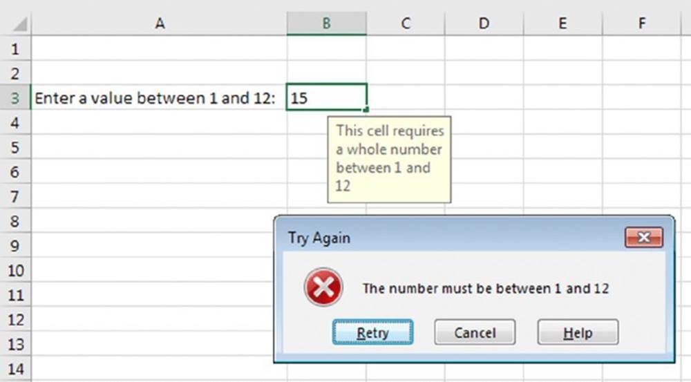
Figure 20.1 Displaying an input message and a message when the user makes an invalid entry.
Excel makes it easy to specify the validation criteria, and you can also use a formula for more complex criteria.
![]() Caution
Caution
The Excel data validation feature suffers from a potentially serious problem: if the user copies a cell that does not use data validation and pastes it to a cell that does use data validation, the data validation rules are deleted. In other words, the cell then accepts any type of data. This has always been a problem, but Microsoft still hasn’t fixed it in Excel 2016.
Specifying Validation Criteria
To specify the type of data allowable in a cell or range, follow these steps while you refer to Figure 20.2, which shows all three tabs of the Data Validation dialog box:
1. Select the cell or range.
2. Choose Data ➜ Data Tools ➜ Data Validation. Excel displays its Data Validation dialog box.
3. Click the Settings tab.
4. Choose an option from the Allow drop-down list. The contents of the Data Validation dialog box will change, displaying controls based on your choice. To specify a formula, select Custom.
5. Specify the conditions by using the displayed controls. Your selection in step 4 determines what other controls you can access.
6. (Optional) Click the Input Message tab and specify which message to display when a user selects the cell. You can use this optional step to tell the user what type of data is expected. If this step is omitted, no message will appear when the user selects the cell.
7. (Optional) Click the Error Alert tab and specify which error message to display when a user makes an invalid entry. The selection for Style determines what choices users have when they make invalid entries. To prevent an invalid entry, choose Stop. If this step is omitted, a standard message will appear if the user makes an invalid entry.
![]() Caution
Caution
Even with data validation in effect, a user can enter invalid data. If the Style setting on the Error Alert tab of the Data Validation dialog box is set to anything except Stop, invalid data can be entered. You can identify invalid entries by having Excel circle them (explained later).
8. Click OK. The cell or range contains the validation criteria you specified.
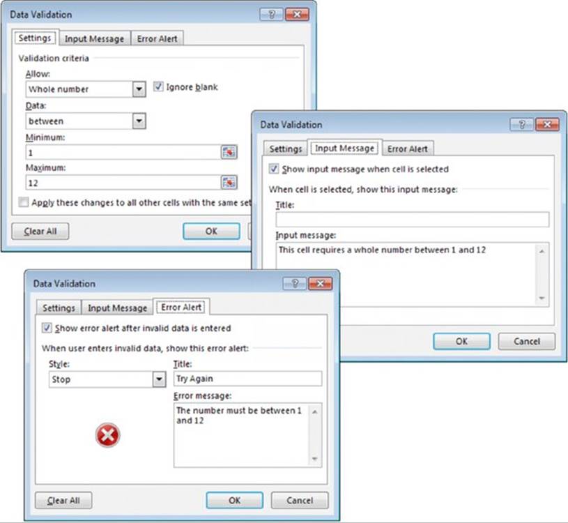
Figure 20.2 The three tabs of the Data Validation dialog box.
![]() Tip
Tip
You can use the optional Input Message with a criteria of Any Value. This allows you to display a message to the user even for cells whose value you don’t want to restrict.
Types of Validation Criteria You Can Apply
From the Settings tab of the Data Validation dialog box, you can specify a variety of data validation criteria. The following options are available from the Allow drop-down list. Keep in mind that the other controls on the Settings tab vary, depending on your choice from the Allow drop-down list.
§ Any Value: Selecting this option removes any existing data validation. Note, however, that the input message, if any, still displays if the check box is selected on the Input Message tab.
§ Whole Number: The user must enter a whole number. You specify a valid range of whole numbers by using the Data drop-down list. For example, you can specify that the entry must be a whole number greater than or equal to 100.
§ Decimal: The user must enter a number. You specify a valid range of numbers by refining the criteria from choices in the Data drop-down list. For example, you can specify that the entry must be greater than or equal to 0 and less than or equal to 1.
§ List: The user must choose from a list of entries you provide. This option is useful, and we discuss it in detail later in this chapter. (See “Creating a Drop-Down List.”)
§ Date: The user must enter a date. You specify a valid date range from choices in the Data drop-down list. For example, you can specify that the entered data must be greater than or equal to January 1, 2016, and less than or equal to December 31, 2016.
§ Time: The user must enter a time. You specify a valid time range from choices in the Data drop-down list. For example, you can specify that the entered data must be later than 12:00 p.m.
§ Text Length: The length of the data (number of characters) is limited. You specify a valid length by using the Data drop-down list. For example, you can specify that the length of the entered data be 1 (a single alphanumeric character).
§ Custom: To use this option, you must supply a logical formula that determines the validity of the user’s entry. (A logical formula returns either TRUE or FALSE.) You can enter the formula directly into the Formula control (which appears when you select the Custom option), or you can specify a cell reference that contains a formula. This chapter contains examples of useful formulas.
![]() Tip
Tip
All the data validation criteria can accept typed values or references to cells. For instance, you can type 1 and 12 to limit whole numbers, or you can point to cells that contain the values 1 and 12.
The Settings tab of the Data Validation dialog box contains two other check boxes:
§ Ignore Blank: If selected, blank entries are allowed.
§ Apply These Changes to All Other Cells with the Same Setting: If selected, the changes you make apply to all other cells that contain the original data validation criteria.
![]() Tip
Tip
The Data ➜ Data Tools ➜ Data Validation drop-down list contains an item labeled Circle Invalid Data. When you select this item, circles appear around cells that contain incorrect entries. If you correct an invalid entry, the circle disappears. To get rid of the circles, choose Data ➜ Data Tools ➜ Data Validation ➜ Clear Validation Circles. In Figure 20.3, invalid entries are defined as values that are less than 1 or greater than 100.
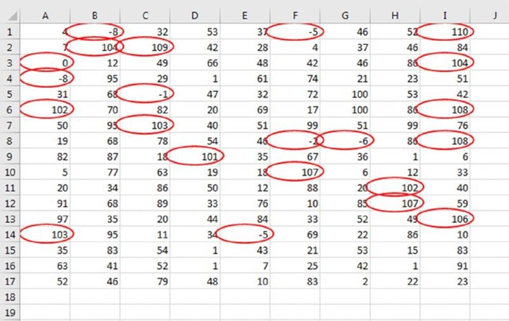
Figure 20.3 Excel can draw circles around invalid entries (in this case, cells that contain values less than 1 or greater than 100).
Creating a Drop-Down List
Perhaps one of the most common uses of data validation is to create a drop-down list in a cell. Figure 20.4 shows an example that uses the month names in A1:A12 as the list source.
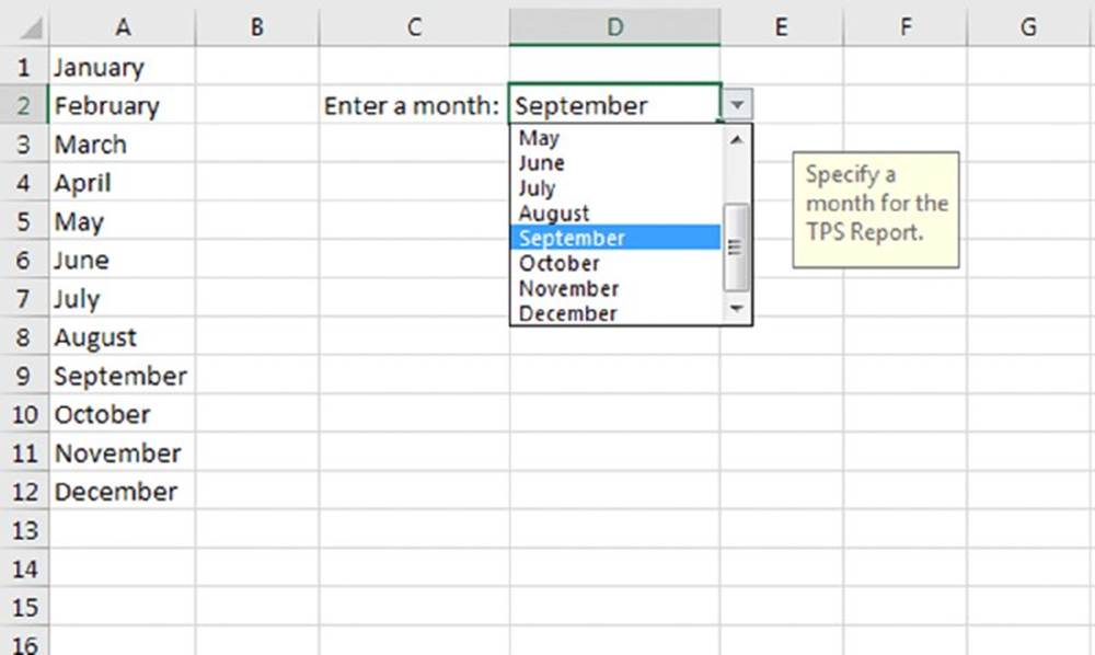
Figure 20.4 This drop-down list (with an Input Message) was created using data validation.
To create a drop-down list in a cell, do the following:
1. Enter the list items into a single-row or single-column range. These items will appear in the drop-down list.
2. Select the cell that will contain the drop-down list and then access the Data Validation dialog box. (Choose Data ➜ Data Tools ➜ Data Validation.)
3. From the Settings tab, select the List option (from the Allow drop-down list) and specify the range that contains the list, using the Source control. The range can be in a different worksheet but must be in the same workbook.
4. Make sure that the In-Cell Dropdown check box is selected.
5. Set any other Data Validation options as desired.
6. Click OK. The cell displays an input message (if specified) and a drop-down arrow when it’s activated. Click the arrow and choose an item from the list that appears.
![]() Tip
Tip
If you have a short list, you can enter the items directly into the Source control of the Settings tab of the Data Validation dialog box. (This control appears when you choose the List option in the Allow drop-down list.) Just separate each item with list separators specified in your regional settings (a comma if you use the U.S. regional settings).
Using Formulas for Data Validation Rules
For simple data validation, the data validation feature is quite straightforward and easy to use. The real power of this feature, though, becomes apparent when you use data validation formulas.
![]() Note
Note
The formula that you specify must be a logical formula that returns either TRUE or FALSE. If the formula evaluates to TRUE, the data is considered valid and remains in the cell. If the formula evaluates to FALSE, a message box appears that displays the message you specify on the Error Alert tab of the Data Validation dialog box. Specify a formula in the Data Validation dialog box by selecting the Custom option from the Allow drop-down list of the Settings tab. Enter the formula directly into the Formula control or enter a reference to a cell that contains a formula. The Formula control appears on the Setting tab of the Data Validation dialog box when the Custom option is selected.
We present several examples of formulas used for data validation in the upcoming section “Data Validation Formula Examples.”
Understanding Cell References
If the formula that you enter into the Data Validation dialog box contains a cell reference, that reference is considered a relative reference, based on the upper-left cell in the selected range.
The following example clarifies this concept. Suppose that you want to allow only an odd number to be entered into the range B2:B10. None of the Excel data validation rules can limit entry to odd numbers, so a formula is required.
Follow these steps:
1. Select the range (B2:B10 for this example) and ensure that cell B2 is the active cell.
2. Choose Data ➜ Data Tools ➜ Data Validation. The Data Validation dialog box appears.
3. Click the Settings tab and select Custom from the Allow drop-down list.
4. Enter the following formula in the Formula field, as shown in Figure 20.5:
=ISODD(B2)
This formula uses the ISODD function, which returns TRUE if its numeric argument is an odd number. Notice that the formula refers to the active cell, which is cell B2.
5. On the Error Alert tab, choose Stop for the Style and then type An odd number is required here as the error message.
6. Click OK to close the Data Validation dialog box.
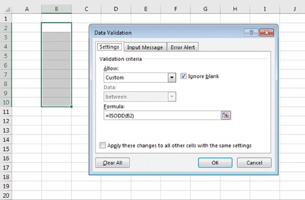
Figure 20.5 Entering a data validation formula.
Notice that the formula entered contains a reference to the upper-left cell in the selected range. This data validation formula was applied to a range of cells, so you might expect that each cell would contain the same data validation formula. Because you entered a relative cell reference as the argument for the ISODD function, Excel adjusts the formula for the other cells in the B2:B10 range. To demonstrate that the reference is relative, select cell B5 and examine its formula displayed in the Data Validation dialog box. You’ll see that the formula for this cell is
=ISODD(B5)
Generally, when entering a data validation formula for a range of cells, you use a reference to the active cell, which is normally the upper-left cell in the selected range. An exception is when you need to refer to a specific cell. For example, suppose that you select range A1:B10 and you want your data validation to allow only values that are greater than the value in cell C1. You would use this formula:
=A1>$C$1
In this case, the reference to cell C1 is an absolute reference; it will not be adjusted for the cells in the selected range, which is just what you want. The data validation formula for cell A2 looks like this:
=A2>$C$1
The relative cell reference is adjusted, but the absolute cell reference is not.
Data Validation Formula Examples
The following sections contain a few data validation examples that use a formula entered directly into the Formula control on the Settings tab of the Data Validation dialog box. These examples help you understand how to create your own data validation formulas.
![]() On the Web
On the Web
All the examples in this section are available at this book’s website. The file is named data validation examples.xlsx.
Accepting text only
Excel has a data validation option to limit the length of text entered into a cell, but it doesn’t have an option to force text (rather than a number) into a cell. To force a cell or range to accept only text (no values), use the following data validation formula:
=ISTEXT(A1)
This formula assumes that the active cell in the selected range is cell A1.
Accepting a larger value than the previous cell
The following data validation formula enables the user to enter a value only if it’s greater than the value in the cell directly above it:
=A2>A1
This formula assumes that A2 is the active cell in the selected range. Note that you can’t use this formula for a cell in row 1.
Accepting nonduplicate entries only
The following data validation formula does not permit the user to make a duplicate entry in the range A1:C20:
=COUNTIF($A$1:$C$20,A1)=1
This is a logical formula that returns TRUE if the value in the cell occurs only one time in the A1:C20 range. Otherwise, it returns FALSE, and the Duplicate Entry dialog box is displayed.
This formula assumes that A1 is the active cell in the selected range. Note that the first argument for COUNTIF is an absolute reference. The second argument is a relative reference, and it adjusts for each cell in the validation range. Figure 20.6 shows this validation criterion in effect, using a custom error alert message. The user is attempting to enter a value into cell B5 that already exists in the A1:C20 range.
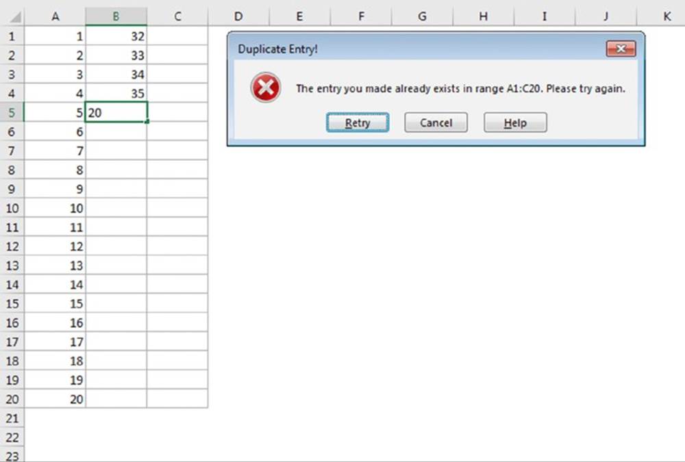
Figure 20.6 Using data validation to prevent duplicate entries in a range.
Accepting text that begins with a specific character
The following data validation formula demonstrates how to check for a specific character. In this case, the formula ensures that the user’s entry is a text string that begins with the letter A (uppercase or lowercase):
=LEFT(A1)="a"
This is a logical formula that returns TRUE if the first character in the cell is the letter A. Otherwise, it returns FALSE. This formula assumes that the active cell in the selected range is cell A1.
If case sensitivity is important and you want to limit entries to only those that start with a lowercase a, you can use the EXACT worksheet function as shown here:
=EXACT(LEFT(A1,1),"a")
The following formula is a variation of the non–case sensitive validation formula. It uses wildcard characters in the second argument of the COUNTIF function. In this case, the formula ensures that the entry begins with the letter A and contains exactly five characters:
=COUNTIF(A1,"A????")=1
Accepting dates by the day of the week
The following data validation formula ensures that the cell entry is a date and that the date is a Monday:
=WEEKDAY(A1)=2
This formula assumes that the active cell in the selected range is cell A1. It uses the WEEKDAY function, which returns 1 for Sunday, 2 for Monday, and so on.
Accepting only values that don’t exceed a total
Figure 20.7 shows a simple budget worksheet, with the budget item amounts in the range B1:B6. The planned budget is in cell E5, and the user is attempting to enter a value in cell B4 that would cause the total (cell E6) to exceed the budget. The following data validation formula ensures that the sum of the budget items does not exceed the budget:
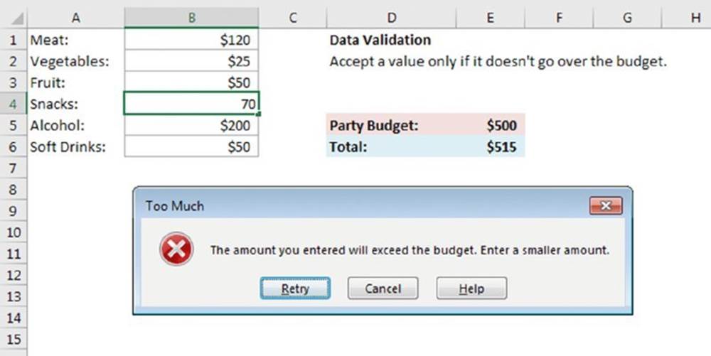
Figure 20.7 Using data validation to ensure that the sum of a range does not exceed a certain value.
=SUM($B$1:$B$6)<=$E$5
Creating a dependent list
As we described previously, you can use data validation to create a drop-down list in a cell (see “Creating a Drop-Down List”). This section explains how to use a drop-down list to control the entries that appear in a second drop-down list. In other words, the second drop-down list is dependent upon the value selected in the first drop-down list.
Figure 20.8 shows a simple example of a dependent list created by using data validation. Cell E2 contains data validation that displays a three-item list from the range A1:C1 (Vegetables, Fruits, and Meats). When the user chooses an item from the list, the second list (in cell F2) displays the appropriate items. Cell E2 contains data validation with its Allow criterion set to List and its Source criterion shown below:
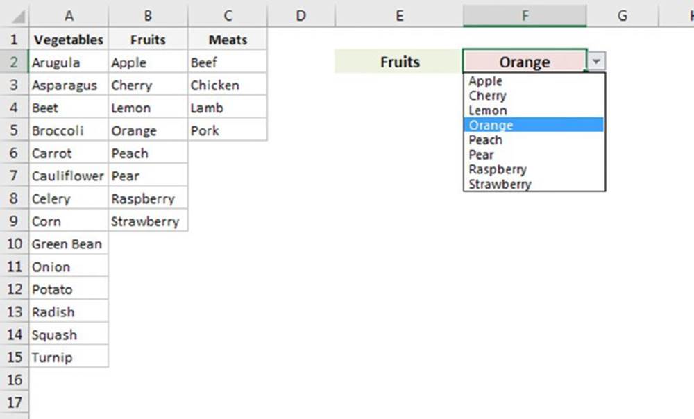
Figure 20.8 The items displayed in the list in cell F2 depend on the list item selected in cell E2.
=$A$1:$C$1
This worksheet uses three named ranges:
§ Vegetables: A2:A15
§ Fruits: B2:B9
§ Meats: C2:C5
For this technique to work, your range names must match the values in A1:C1. For example, if you type Veggies in cell A1 and name the range Vegetables, the list in F2 won’t contain items. Cell F2 contains data validation that uses this formula:
=INDIRECT($E$2)
The INDIRECT function converts its argument into a range if it can. If cell E2 contains the text Fruits, for instance, INDIRECT looks for a range named Fruits and supplies that range to the data validation list.
![]() Caution
Caution
Dependent data validation lists have a flaw. If you select a fruit from the list (see Figure 20.8) and then change cell E2 to Meats, the value you selected in F2 will become invalid. The only way you’ll know this is if you pull down the list in F2 or circle invalid data.
Using Structured Table Referencing
With Excel Tables (Insert ➜ Table) you can use structured table referencing in your formulas. Figure 20.9 shows a simple table consisting of one column of names. You can create a formula like this one that matches a name to the list:
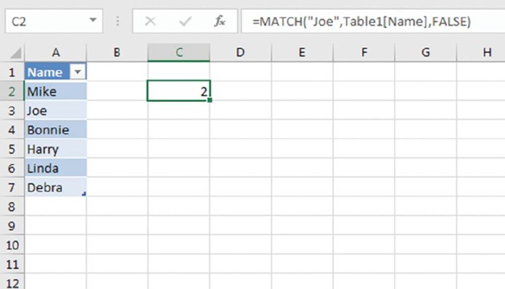
Figure 20.9 Structured references grow or shrink with the table.
=MATCH("Joe",Table1[Name],FALSE)
The second argument, Table1[Name], is a structured reference that returns the Name column of the table named Table1. As you add or remove rows to that table, the structured reference adjusts and your formulas continue to work.
![]() Cross-Ref
Cross-Ref
See Chapter 9, “Working with Tables and Lists,” for more information on structured table references.
Unfortunately, you can’t use structured table references in your data validation criteria. To overcome this, you can create a named range that uses a structured table reference and use that name in your data validation.
To create a named range, choose Formulas ➜ Defined Names ➜ Define Name for the Ribbon. Enter the name, such as dvTable1Name, and point to the table’s column in the Refers To box. The reference changes to =Table1[Name], as shown in Figure 20.10.
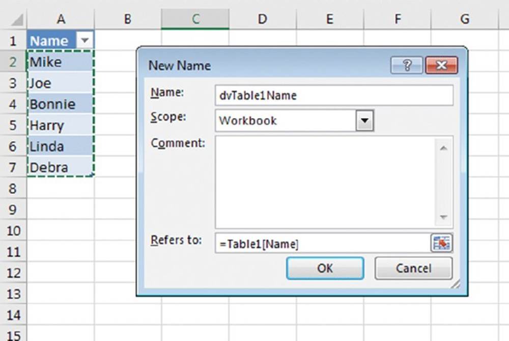
Figure 20.10 Named ranges can refer to tables using structured references.
Now you can use dvTable1Name in your data validation to get a list that grows or shrinks with the table. Figure 20.11 shows a cell with such validation.
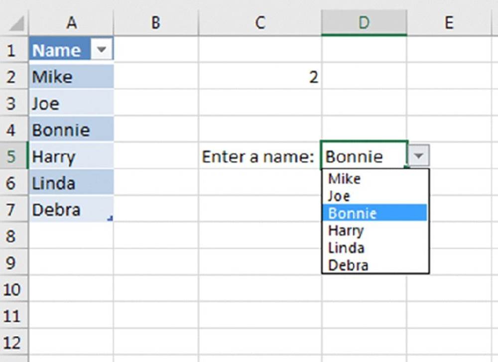
Figure 20.11 A defined name can be used in data validation to avoid the structured reference limitation.
This example used a naming convention of dv plus the table name plus the column name. You don’t have to use a convention like this; you can use any valid named range.
All materials on the site are licensed Creative Commons Attribution-Sharealike 3.0 Unported CC BY-SA 3.0 & GNU Free Documentation License (GFDL)
If you are the copyright holder of any material contained on our site and intend to remove it, please contact our site administrator for approval.
© 2016-2026 All site design rights belong to S.Y.A.