Excel 2016 Formulas (2016)

PART V
Miscellaneous Formula Techniques

Chapter 21
Creating Megaformulas

In This Chapter

· What a megaformula is and why you would want to use such a thing

· How to create a megaformula

· Examples of megaformulas

· How to use named formulas to create a megaformula

· Pros and cons of using megaformulas

This chapter describes a useful technique that combines several formulas into a single formula—what we call a megaformula. This technique can eliminate intermediate formulas and may even speed up recalculation. The downside, as you’ll see, is that the resulting formula is virtually incomprehensible and may be impossible to edit.

What Is a Megaformula?

Often, a worksheet may require intermediate formulas to produce a desired result. In other words, a formula may depend on other formulas, which in turn depend on other formulas. After you get all these formulas working correctly, you often can eliminate the intermediate formulas and create a single (and more complex) formula. For lack of a better term, we call such a formula a megaformula.

What are the advantages of employing megaformulas? They use fewer cells (less clutter), and recalculation may be faster. And you can impress people in the know with your formula-building abilities. The disadvantages? The formula probably will be impossible to decipher or modify, even by the person who created it.

Note

We use the techniques described in this chapter to create many of the complex formulas presented elsewhere in this book.

Using megaformulas is actually a rather controversial issue. Some claim that the clarity that results from having multiple formulas far outweighs any advantages in having a single incomprehensible formula. You can decide for yourself.

Creating a Megaformula: A Simple Example

Creating a megaformula basically involves copying formula text and pasting it into another formula. We start with a relatively simple example. Examine the spreadsheet shown in Figure 21.1. This sheet uses formulas to calculate mortgage loan information.

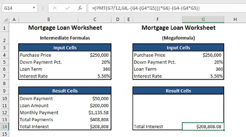
Figure 21.1 This spreadsheet uses multiple formulas to calculate mortgage loan information.

On the Web

This workbook, named total interest.xlsx, is available at this book’s website.

The Result Cells section of the worksheet uses information entered into the Input Cells section and contains the formulas shown in Table 21.1.

Table 21.1 Formulas Used to Calculate Total Interest

Suppose you’re really interested in the total interest paid (cell C14). You could, of course, simply hide the rows that contain the extraneous information. However, it’s also possible to create a single formula that does the work of several intermediary formulas.

Note

This example is for illustration only. The CUMIPMT function provides a more direct way to calculate total interest on a loan.

The formula that calculates total interest depends on the formulas in cells C11 and C13 (which are the direct precedent cells). In addition, the formula in cell C13 depends on the formula in cell C12. And cell C12, in turn, depends on cell C11. Therefore, calculating the total interest in this example uses five formulas. The steps that follow describe how to create a single formula to calculate total interest so that you can eliminate the four intermediate formulas.

C14 contains the following formula:

=C13-C11

The steps that follow describe how to convert this formula into a megaformula:

1. Substitute the formula contained in cell C13 for the reference to cell C13.

Before doing this, add parentheses around the formula in C13. (Without the parentheses, the calculations occur in the wrong order.) Now the formula in C14 is

=(C12*C6)-C11

2. Substitute the formula contained in cell C12 for the reference to cell C12. Now the formula in C14 is

=(PMT(C7/12,C6,-C11)*C6)-C11

3. Substitute the formula contained in cell C11 for the two references to cell C11. Before copying the formula, you need to insert parentheses around it. Now the formula in C14 is

=(PMT(C7/12,C6,-(C4-C10))*C6)-(C4-C10)

4. Substitute the formula contained in cell C10 for the two references to cell C10. Before copying the formula, insert parentheses around it. Now the formula in C14 is

=(PMT(C7/12,C6,-(C4-(C4*C5)))*C6)-(C4-(C4*C5))

At this point, the formula contains references only to input cells. The formulas in range C10:C13 are not referenced, so you can delete them. The single megaformula now does the work previously performed by the intermediary formulas.

Unless you’re a world-class Excel formula wizard, it’s quite unlikely that you could arrive at that formula without first creating intermediate formulas.

Creating a megaformula essentially involves substituting formula text for cell references in a formula. You perform substitutions until the megaformula contains no references to formula cells. At each step along the way, you can check your work by ensuring that the formula continues to display the same result. In the previous example, a few of the steps required parentheses around the copied formula to ensure the correct order of calculation.

Copying text from a formula

Creating megaformulas involves copying formula text and then replacing a cell reference with the copied text. To copy the contents of a formula, activate the cell and press F2. Select the formula text (without the equal sign) by pressing Shift+Home, followed by Shift+right arrow. Press Ctrl+C to copy the selected text to the Clipboard, and then press Esc to cancel cell editing. Activate the cell that contains the megaformula and press F2. Use the arrow keys, and hold down Shift to select the cell reference that you want to replace. Finally, press Ctrl+V to replace the selected text with the Clipboard contents.

In some cases, you need to insert parentheses around the copied formula text to make the formula calculate correctly. If the formula returns a different result after you paste the formula text, press Ctrl+Z to undo the paste. Insert parentheses around the formula you want to copy and paste it into the megaformula. It should then calculate correctly.

Megaformula Examples

This section contains three additional examples of megaformulas. These examples provide a thorough introduction to applying the megaformula technique for streamlining a variety of tasks, including cleaning up a list of names by removing middle names and initials, returning the position of the last space character in a string, determining whether a credit card number is valid, and generating a list of random names.

Using a megaformula to remove middle names

Consider a worksheet with a column of names, like the one shown in Figure 21.2. Suppose you have a worksheet with thousands of such names, and you need to remove all the middle names and middle initials from the names. Editing the cells manually would take hours, and you’re not up to writing a VBA macro, so that leaves using a formula-based solution. Notice that not all the names have a middle name or a middle initial, which makes the task a bit trickier. Although this is not a difficult task, it normally involves several intermediate formulas.

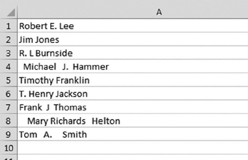
Figure 21.2 The goal is to remove the middle name or middle initial from each name.

Cross-Ref

The Flash Fill feature, introduced in Excel 2013, can handle this task without using formulas. See Chapter 16, “Importing and Cleaning Data,” for more information about Flash Fill.

Figure 21.3 shows the results of the more conventional solution, which requires six intermediate formulas, as shown in Table 21.2. The names are in column A; column H displays the end result. Columns B:G hold the intermediate formulas.

Table 21.2 Intermediate Formulas in the First Row of Sheet1 in Figure 21.3

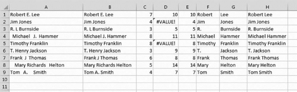
Figure 21.3 Removing the middle names and initials requires six intermediate formulas.

On the Web

You can access the workbook for removing middle names and initials at this book’s website. The filename is no middle name.xlsx.

Note that cell E1 uses the IFERROR function, which was introduced in Excel 2007. For compatibility with earlier versions, use this formula:

=IF(ISERROR(D1),C1,D1)

Note

Notice that the result isn’t perfect. For example, it will not work if the cell contains only one name (for example, Enya). This method also fails if a name has two middle names (such as John Jacob Robert Smith). That occurs because the formula simply searches for the second space character in the name. In this example, the megaformula returns John Robert Smith. Later in this chapter, we present an array formula method to identify the last space character in a string.

With a bit of work, you can eliminate all the intermediate formulas and replace them with a single megaformula. You do so by creating all the intermediate formulas and then editing the final result formula (in this case, the formula in column H) by replacing each cell reference with a copy of the formula in the cell referred to. Fortunately, you can use the Clipboard to copy and paste. (See the sidebar “Copying text from a formula,” earlier in this chapter.) Keep repeating this process until cell H1 contains nothing but references to cell A1. You end up with the following megaformula in one cell:

=LEFT(TRIM(A1),FIND(" ",TRIM(A1))–1)&" "&RIGHT

(TRIM(A1),LEN(TRIM(A1))–IFERROR(FIND(" ",TRIM(A1),

FIND(" ",TRIM(A1))+1),FIND(" ",TRIM(A1))))

When you’re satisfied that the megaformula works, you can delete the columns that hold the intermediate formulas because they are no longer used.

The step-by-step procedure

If you’re still not clear about this process, take a look at the step-by-step procedure:

1. Examine the formula in H1. This formula contains two cell references (F1 and G1):

=F1&" "&G1

2. Activate cell G1 and copy the contents of the formula (without the equal sign) to the Clipboard.

3. Activate cell H1 and replace the reference to cell G1 with the Clipboard contents.

Now cell H1 contains the following formula:

=F1&" "&RIGHT(B1,LEN(B1)–E1)

4. Activate cell F1 and copy the contents of the formula (without the equal sign) to the Clipboard.

5. Activate cell H1 and replace the reference to cell F1 with the Clipboard contents.

Now the formula in cell H1 is as follows:

=LEFT(B1,C1–1)&" "&RIGHT(B1,LEN(B1)–E1)

6. Cell H1 contains references to three cells (B1, C1, and E1).

The formulas in those cells will replace each of the three references.

7. Replace the reference to cell E1 with the formula in cell E1. The result is

=LEFT(B1,C1–1)&" "&RIGHT(B1,LEN(B1)–IFERROR(D1,C1))

8. Replace the reference to cell D1 with the formula in cell D1.

The formula now looks like this:

=LEFT(B1,C1–1)&" "&RIGHT(B1,LEN(B1)–IFERROR(FIND(" ",B1,C1+1),C1))

9. The formula has three references to cell C1. Replace all three of those references to cell C1 with the formula contained in cell C1.

The formula in cell H1 is as follows:

=LEFT(B1,FIND(" ",B1)–1)&" "&RIGHT(B1,LEN(B1)–IFERROR

(FIND(" ",B1,FIND(" ",B1)+1),FIND(" ",B1)))

10. Finally, replace the seven references to cell B1 with the formula in cell B1. The result is

11. =LEFT(TRIM(A1),FIND(" ",TRIM(A1))–1)&" "&RIGHT

12. (TRIM(A1),LEN(TRIM(A1))–IFERROR(FIND(" ",TRIM(A1),

FIND(" ",TRIM(A1))+1),FIND(" ",TRIM(A1))))

Notice that the formula in cell H1 now contains references only to cell A1. The megaformula is complete, and it performs exactly the same tasks as all the intermediate formulas (which you can now delete).

After you create a megaformula, you can create a name for it to simplify using the formula. Here’s an example:

1. Copy the megaformula text to the Clipboard.

In this example, the megaformula refers to cell A1.

2. Activate cell B1, which is the cell to the right of the cell referenced in the megaformula.

3. Choose Formulas ➜ Defined Names ➜ Define Name to display the New Name dialog box.

4. In the Name field, type NoMiddleName.

5. Activate the Refers To field and press Ctrl+V to paste the megaformula text.

6. Click OK to close the New Name dialog box.

After performing these steps and creating the named formula, you can enter the following formula, and it will return the result using the cell directly to the left:

=NoMiddleName

If you enter this formula in cell K8, it displays the name in cell J8, with no middle name.

Cross-Ref

See Chapter 3, “Working with Names,” for more information about creating and using named formulas.

This megaformula uses the IFERROR function, so it will not work with versions prior to Excel 2007. A comparable formula that’s compatible with previous versions follows:

=LEFT(TRIM(A1),FIND(" ",TRIM(A1),1)–1)&" "&RIGHT

(TRIM(A1),LEN(TRIM(A1))–IF(ISERROR(FIND(" ",TRIM(A1),

FIND(" ",TRIM(A1),1)+1)),FIND(" ",TRIM(A1),1),FIND(" ",TRIM

(A1),FIND(" ",TRIM(A1),1)+1)))

Comparing speed and efficiency

Because a megaformula is so complex, you may think that using one slows down recalculation. Actually, that’s not the case. As a test, we created three workbooks (each with 175,000 names): one that used six intermediate formulas, one that used a megaformula, and one that used a named megaformula. We compared the results in terms of calculation time and file size; see Table 21.3.

Table 21.3 Comparing Intermediate Formulas and Megaformulas

Of course, the actual results will vary depending on your system’s processor speed.

As you can see, using a megaformula (or a named megaformula) in this case resulted in slightly faster recalculations as well as a much smaller workbook.

On the Web

The three test workbooks that we used are available at this book’s website. The filenames are time test intermediate.xlsx, time test megaformula.xlsx, and time test named megaformula.xlsx. To perform your own time tests, change the name in cell A1 and start your stopwatch when you press Enter. Keep your eye on the status bar, which indicates when the calculation is finished.

Using a megaformula to return a string’s last space character position

As previously noted, the “remove middle name” example presented earlier contains a flaw: to identify the last name, the formula searches for the second space character. A better solution is to search for the last space character. Unfortunately, Excel doesn’t provide a simple way to locate the position of the first occurrence of a character from the end of a string. The example in this section solves that problem and describes a way to determine the position of the first occurrence of a specific character going backward from the end of a text string.

Cross-Ref

This technique involves arrays, so you might want to review the material in Part IV, “Array Formulas,” to familiarize yourself with this topic.

This example describes how to create a megaformula that returns the character position of the last space character in a string. You can, of course, modify the formula to work with any other character.

Creating the intermediate formulas

The general plan is to create an array of characters in the string, but in reverse order. After that array is created, you can use the MATCH function to locate the first space character in the array.

Refer to Figure 21.4, which shows the results of the intermediate formulas. Cell A1 contains an arbitrary name, which happens to use 12 characters. The range B1:B12 contains the following array formula:

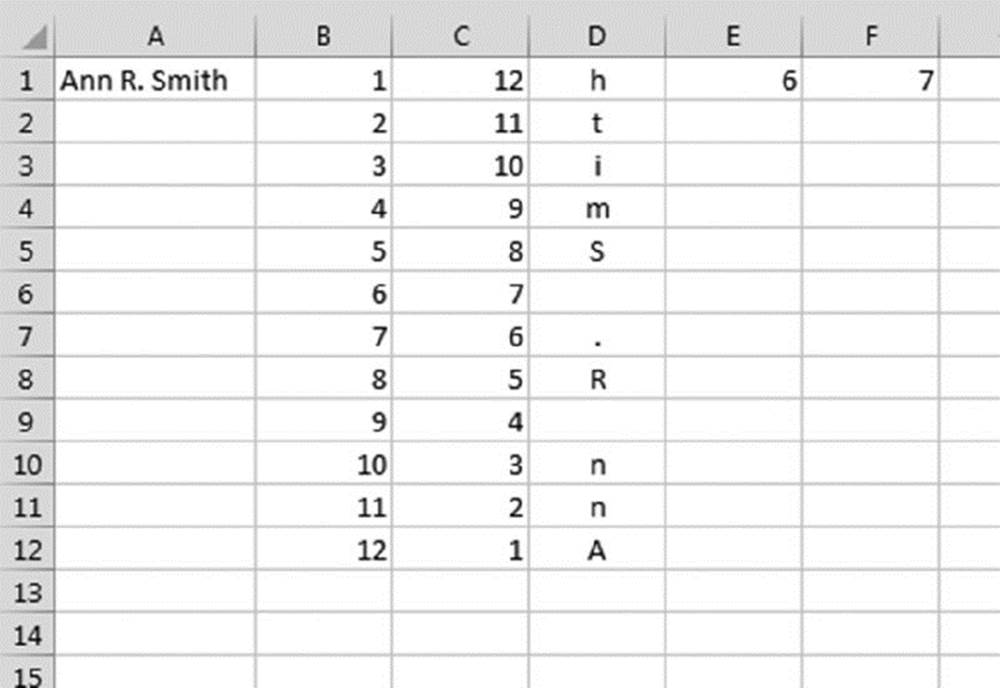
Figure 21.4 These intermediate formulas will eventually be converted to a single megaformula.

{=ROW(INDIRECT("1:"&LEN(A1)))}

On the Web

This example, named position of last space.xlsx, is available at this book’s website.

You enter this multicell array formula into the entire B1:B12 range by selecting the range, typing the formula, and pressing Ctrl+Shift+Enter. Don’t type the curly brackets. Excel adds the curly brackets to indicate an array formula. This formula returns an array of 12 consecutive integers.

The range C1:C12 contains the following array formula:

{=LEN(A1)+1–B1:B12}

This formula reverses the integers generated in column B.

The range D1:D12 contains the following array formula:

{=MID(A1,C1:C12,1)}

This formula uses the MID function to extract the individual characters in cell A1. The MID function uses the array in C1:C12 as its second argument. The result is an array of the name’s characters in reverse order.

The formula in cell E1 is as follows:

=MATCH(" ",D1:D12,0)

This formula, which is not an array formula, uses the MATCH function to return the position of the first space character in the range D1:D12. In the example shown in Figure 21.4, the formula returns 6, which means that the first space character is six characters from the end of the text in cell A1.

The formula in cell F1 follows:

=LEN(A1)+1–E1

This formula returns the character position of the last space in the string.

You may wonder how all these formulas can possibly be combined into a single formula. Keep reading for the answer.

Creating the megaformula

At this point, cell F1 contains the result that you’re looking for—the number that indicates the position of the last space character. The challenge is consolidating all those intermediate formulas into a single formula. The goal is to produce a formula that contains only references to cell A1. These steps will get you to that goal:

1. The formula in cell F1 contains a reference to cell E1. Replace that reference with the text of the formula in cell E1.

As a result, the formula in cell F1 becomes this:

=LEN(A1)+1–MATCH(" ",D1:D12,0)

2. The formula contains a reference to D1:D12. This range contains a single array formula.

Replacing the reference to D1:D12 with the array formula results in the following array formula in cell F1:

{=LEN(A1)+1–MATCH(" ",MID(A1,C1:C12,1),0)}

Note

Because an array formula replaced the reference in cell F1, you must now enter the formula in F1 as an array formula (enter by pressing Ctrl+Shift+Enter).

3. The formula in cell F1 contains a reference to C1:C12, which also contains an array formula. Replace the reference to C1:C12 with the array formula in C1:C12 to get this array formula in cell F1:

{=LEN(A1)+1–MATCH(" ",MID(A1,LEN(A1)+1–B1:B12,1),0)}

4. Replace the reference to B1:B12 with the array formula in B1:B12. The result is

{=LEN(A1)+1–MATCH(" ",MID(A1,LEN(A1)+1–ROW(INDIRECT ("1:"&LEN(A1))),1),0)}

Now the array formula in cell F1 refers only to cell A1, which is exactly what you want. The megaformula does the job, and you can delete all the intermediate formulas.

Note

Although you use a 12-digit value and arrays stored in 12-row ranges to create the formula, the final formula does not use any of these range references. Consequently, the megaformula works with text of any length.

Putting the megaformula to work

Figure 21.5 shows a worksheet with names in column A. Column B contains the megaformula developed in the previous section. Column C contains a formula that extracts the characters beginning after the last space, which represents the last name of the name in column A.

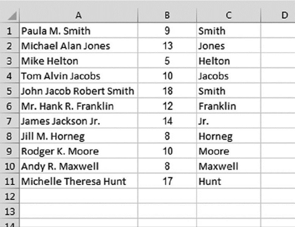
Figure 21.5 Column B contains a megaformula that returns the character position of the last space of the name in column A.

Cell C1, for example, contains this formula:

=RIGHT(A1,LEN(A1)–B1)

If you like, you can eliminate the formulas in column B and create a specialized formula that returns the last name. To do so, substitute the formula in cell B1 for the reference to cell B1 in the formula. The result is the following array formula:

{=RIGHT(A1,LEN(A1)–(LEN(A1)+1–MATCH(" ",MID(A1,LEN(A1)+

1–ROW(INDIRECT("1:"&LEN(A1))),1),0)))}

Note

You must insert parentheses around the formula text copied from cell B1. Without the parentheses, the formula does not evaluate correctly.

Using a megaformula to determine the validity of a credit card number

Many people are not aware that you can determine the validity of a credit card number by using a relatively complex algorithm to analyze the digits of the number. In addition, you can determine the type of credit card by examining the initial digits and the length of the number. Table 21.4 shows information about four major credit cards.

Table 21.4 Information About Four Major Credit Cards

Note

Validity, as used here, means whether the credit card number itself is a valid number as determined by the following steps. This technique, of course, cannot determine whether the number represents an actual credit card account.

You can test the validity of a credit card account number by processing its checksum. All account numbers used in major credit cards use a Mod 10 check-digit algorithm. The general process is as follows:

1. Add leading zeros to the account number to make the total number of digits equal 16.

2. Beginning with the first digit, double the value of alternate digits of the account number. If the result is a two-digit number, add the two digits together.

3. Add the eight values generated in step 2 to the sum of the skipped digits of the original number.

4. If the sum obtained in step 3 is evenly divisible by 10, the number is a valid credit card number.

The example in this section describes a megaformula that determines whether a credit card number is a valid number.

The basic formulas

Figure 21.6 shows a worksheet set up to analyze a credit card number and determine its validity. This workbook uses quite a few formulas to make the determination.

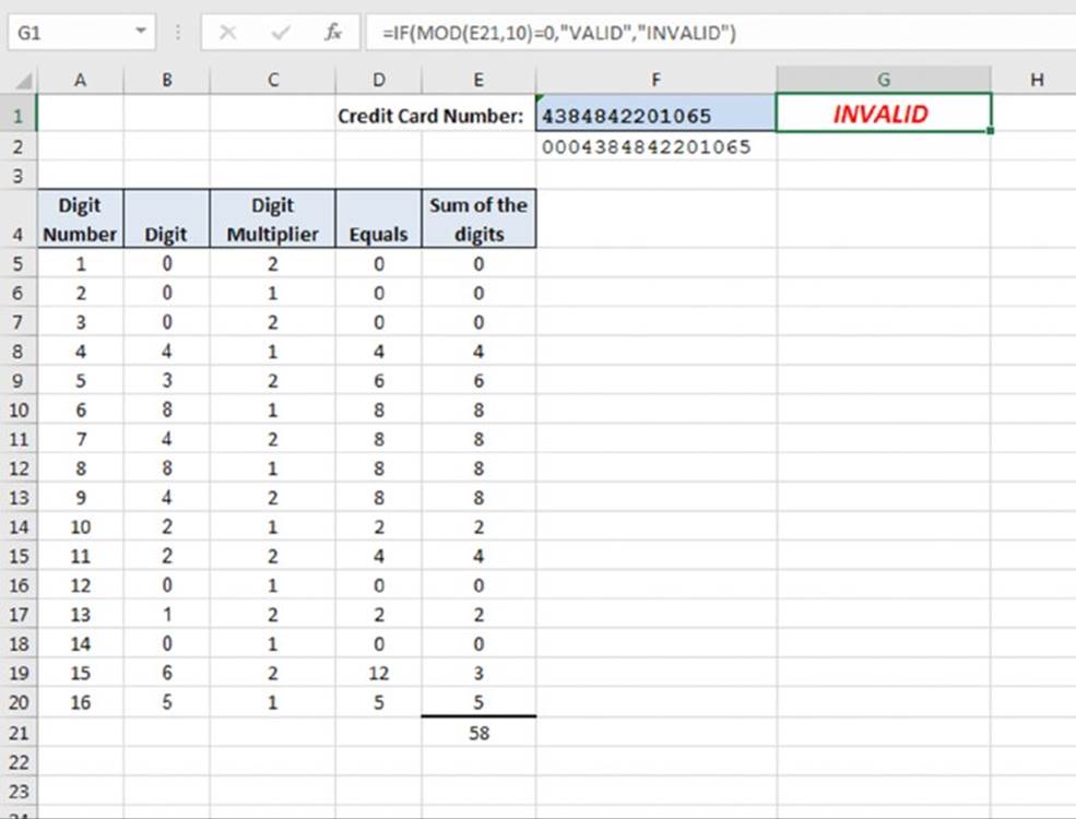
Figure 21.6 The formulas in this worksheet determine the validity of a credit card number.

On the Web

You can access the credit card number validation workbook at this book’s website. The file is named credit card validation.xlsx.

In this worksheet, the credit card number is entered in cell F1, with no spaces or hyphens. The formula in cell F2 follows. This formula appends leading zeros, if necessary, to make the card number exactly 16 digits long. The other formulas use the string in cell F2.

=REPT("0",16–LEN(F1))&F1

Warning

When entering a credit card number that contains more than 15 digits, you must be careful that Excel does not round the number to 15 digits. You can precede the number with an apostrophe or preformat the cell as Text (using Home ➜ Number ➜ Number Format ➜ Text).

Column A contains a series of integers from 1 to 16, each representing the digit positions of the credit card.

Column B contains formulas that extract each digit from cell F2. For example, the formula in cell B5 is as follows:

=MID($F$2,A5,1)

Column C contains the multipliers for each digit: alternating 2s and 1s.

Column D contains formulas that multiply the digit in column B by the multiplier in column C. For example, the formula in cell D5 is

=B5*C5

Column E contains formulas that sum the digits displayed in column D. A single digit value in column D is returned directly. For two-digit values, the sum of the digits is displayed in column E. For example, if column D displays 12, the formula in column E returns 3: that is, 1 + 2. The formula that accomplishes this is as follows:

=INT((D5/10)+MOD((D5),10))

Cell E21 contains a simple SUM formula to add the values in column E:

=SUM(E5:E20)

The formula in cell G1, which follows, calculates the remainder when cell E21 is divided by 10. If the remainder is 0, the card number is valid, and the formula displays VALID. Otherwise, the formula displays INVALID.

=IF(MOD(E21,10)=0,"VALID","INVALID")

Convert to array formulas

The megaformula that performs all these calculations will be an array formula because the intermediary formulas occupy multiple rows.

First, you need to convert all the formulas to array formulas. Note that columns A and C consist of values, not formulas. To use the values in a megaformula, they must be generated by formulas—more specifically, array formulas.

Enter the following array formula into the range A5:A20. This array formula returns a series of 16 consecutive integers:

{=ROW(INDIRECT("1:16"))}

1. For column B, select B5:B20 and enter the following array formula, which extracts the digits from the credit card number:

{=MID($F$2,A5:A20,1)}

2. Column C requires an array formula that generates alternating values of 2 and 1.

Such a formula, entered into the range C5:C20, is shown here:

{=(MOD(ROW(INDIRECT("1:16")),2)+1)}

3. For column D, select D5:D20 and enter the following array formula:

{=B5:B20*C5:C20}

4. Select E5:E20 and enter this array formula:

{=INT((D5:D20/10)+MOD((D5:D20),10))}

Now the worksheet contains five columns of 16 rows but only five actual formulas (which are multicell array formulas).

Build the megaformula

To create the megaformula for this task, start with cell G1, which is the cell that has the final result. The original formula in G1 is

=IF(MOD(E21,10)=0,"VALID","INVALID")

1. Replace the reference to cell E21 with the formula in E21.

Doing so results in the following formula in cell G1:

=IF(MOD(SUM(E5:E20),10)=0,"VALID","INVALID")

2. Replace the reference to E5:E20 with the array formula contained in that range. Now the formula becomes an array formula, so you must enter it by pressing Ctrl+Shift+Enter.

After the replacement, the formula in G1 is as follows:

{=IF(MOD(SUM(INT((D5:D20/10)+MOD((D5:D20),10))),10)=0,

"VALID","INVALID")}

3. Replace the two references to range D5:D20 with the array formula contained in D5:20.

Doing so results in the following array formula in cell G1:

{=IF(MOD(SUM(INT((B5:B20*C5:C20/10)+MOD((B5:B20*C5:C20),

10))),10)=0,"VALID","INVALID")}

4. Replace the references to cell C5:C20 with the array formula in C5:C20.

Note that you must have a set of parentheses around the copied formula text. The result is as follows:

{=IF(MOD(SUM(INT((B5:B20*(MOD(ROW(INDIRECT("1:16")),

2)+1)/10)+MOD((B5:B20*(MOD(ROW(INDIRECT("1:16")),2)+1)),

10))),10)=0,"VALID","INVALID")}

5. Replacing the references to B5:B20 with the array formula contained in B5:B20 yields the following:

6. {=IF(MOD(SUM(INT((MID($F$2,A5:A20,1)*(MOD(ROW(INDIRECT

7. ("1:16")),2)+1)/10)+MOD((MID($F$2,A5:A20,1)*(MOD(ROW

8. (INDIRECT("1:16")),2)+1)),10))),10)

=0,"VALID","INVALID")}

6. Substitute the array formula in range A5:A20 for the references to that range.

The resulting array formula is as follows:

{=IF(MOD(SUM(INT((MID($F$2,ROW(INDIRECT("1:16")),1)*(MOD(ROW

(INDIRECT("1:16")),2)+1)/10)+MOD((MID($F$2,ROW(INDIRECT

("1:16")),1)*(MOD(ROW(INDIRECT("1:16")),2)+1)),10))),10)=0,

"VALID","INVALID")}

7. Substitute the formula in cell F2 for the two references to cell F2.

After making the substitutions, the formula is as follows:

{=IF(MOD(SUM(INT((MID(REPT("0",16–LEN(F1))&F1,

ROW(INDIRECT("1:16")),1)*(MOD(ROW(INDIRECT("1:16")),2)+1)/

10)+MOD((MID(REPT("0",16–LEN(F1))&F1,ROW(INDIRECT("1:16")),

1)*(MOD(ROW(INDIRECT("1:16")),2)+1)),10))),10)=0,"VALID",

"INVALID")}

You can delete the now superfluous intermediate formulas. The final megaformula, a mere 229 characters in length, does the work of 51 intermediary formulas!

Figure 21.7 shows this formula at work.

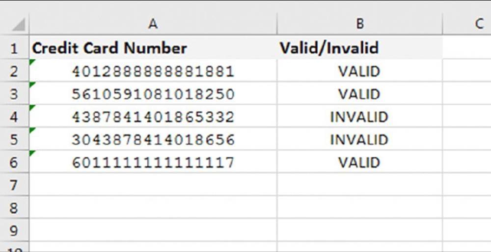
Figure 21.7 Using a megaformula to determine the validity of credit card numbers.

Using Intermediate Named Formulas

One way you can make your mega formulas easier to read is to name them. This technique was described in an earlier section about removing middle names. A variation of this technique is to use several named formulas rather than one named megaformula.

The credit card validation formula could be made to look like this:

=IF(MOD(SUM(SumOfDigits),10)=0,"VALID","INVALID")

There’s still a lot you can’t see in that formula, but it does give you a feel for what the formula is doing, as opposed to a named megaformula, which might look like this:

=IsCreditCardValid

This technique involves creating a series of named formulas. Some of the names will refer to previously created names. Start by creating a name called Padded for this formula:

=REPT("0",16-LEN(INDIRECT("RC[-1]",FALSE)))&INDIRECT("RC[-1]",FALSE)

This simply uses the formula from cell F2 in the previous example, except that it uses INDIRECT and R1C1 notation to refer to the cell just to the left of where this name is used. You could use this named formula as is. Simply type =Padded into a cell with a credit card number in the cell to the left, and it will return the number padded with zeros.

The remaining formulas either refer to Padded, another named formula, or a formula with no cell references. Table 21.5 shows the remaining named formulas.

Table 21.5 Named Formulas to Validate Credit Card Numbers

None of these named formulas refers to a fixed cell, so you can use them in any cell on any worksheet (as long as there’s a cell to the left). If something goes wrong, you can inspect each intermediate named formula to help you troubleshoot the problem.

Generating random names

The final example is a useful application that generates random names. It uses three name lists compiled by the U.S. Census Bureau: 4,275 female first names; 1,219 male first names; and 18,839 last names. The names are sorted by frequency of occurrence. The megaformula selects random names such that more frequently occurring names have a higher probability of being selected. Therefore, if you create a list of random names, they will appear to be somewhat realistic. (Common names will appear more often than uncommon names.)

Figure 21.8 shows the workbook. Cells B7 and B8 contain values that determine the probability that the random name is a male as well as the probability that the random name contains a middle initial. The randomly generated names begin in cell A11.

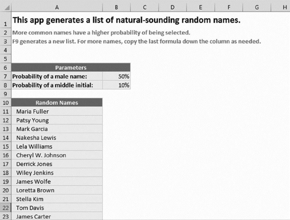
Figure 21.8 This workbook uses a megaformula to generate realistic random names.

On the Web

This workbook, named name generator.xlsx, is available at this book’s website.

The megaformula is as follows. (The workbook uses several names.)

=IF(RAND()<=PctMale,INDEX(MaleNames,MATCH(RAND(),

MaleProbability,–1)),INDEX(FemaleNames,MATCH(RAND(),

FemaleProbability,–1)))&IF(RAND()<=PctMiddle," "&

INDEX(MiddleInitials,MATCH(RAND(),MiddleProbability,–1))&

".","")&" "&INDEX(LastNames,MATCH(RAND(),LastProbability,–1))

We don’t list the intermediate formulas here, but you can examine them by opening the file at this book’s website.

The Pros and Cons of Megaformulas

If you followed the examples in this chapter, you probably realize that the main advantage of creating a megaformula is to eliminate intermediate formulas. Doing so can streamline your worksheet and reduce the size of your workbook files, and it may even result in slightly faster recalculations.

The downside? Creating a megaformula does, of course, require some additional time and effort. And, as you’ve undoubtedly noticed, a megaformula is virtually impossible for anyone (even the author) to figure out. If you decide to use megaformulas, take extra care to ensure that the intermediate formulas are performing correctly before you start building a megaformula. Even better, keep a single copy of the intermediate formulas somewhere in case you discover an error or need to make a change.