Excel 2016 Formulas (2016)

PART V
Miscellaneous Formula Techniques

Chapter 22
Tools and Methods for Debugging Formulas

In This Chapter

· What is formula debugging?

· How to identify and correct common formula errors

· A description of Excel’s auditing tools

Errors happen. And when you create Excel formulas, errors happen frequently. This chapter describes common formula errors and discusses tools and methods that you can use to help create formulas that work as they are intended to.

Formula Debugging?

Debugging refers to identifying and correcting errors in a computer program. Strictly speaking, an Excel formula is not a computer program. Formulas, however, are subject to the same types of problems that occur in a computer program. If you create a formula that does not work as it should, you need to identify and correct the problem.

The ultimate goal in developing a spreadsheet solution is to generate accurate results. For simple worksheets, this is not difficult, and you can usually tell whether the formulas are producing correct results. But as your worksheets grow in size or complexity, ensuring accuracy becomes more difficult.

Making a change in a worksheet—even a relatively minor one—may produce a ripple effect that introduces errors in other cells. For example, accidentally entering a value into a cell that previously held a formula is all too easy to do. This simple error can have a major impact on other formulas, and you may not discover the problem until long after you made the change—or you may never discover the problem.

Research on spreadsheet errors

Using a spreadsheet can be hazardous to your company’s bottom line. It’s tempting to simply assume that your spreadsheet produces accurate results. If you use the results of a spreadsheet to make a major decision, it’s especially important to make sure that the formulas return accurate and meaningful results.

Researchers have conducted quite a few studies that deal with spreadsheet errors. Generally, these studies have found that between 20 and 40 percent of all spreadsheets contain some type of error. If this type of research interests you, check out the European Spreadsheet Risk Interest Group. The URL follows:

http://eusprig.org/

Formula Problems and Solutions

Formula errors tend to fall into one of the following general categories:

§ Syntax errors: You have a problem with the syntax of a formula. For example, a formula may have mismatched parentheses, or a function may not have the correct number of arguments.

§ Logical errors: A formula does not return an error, but it contains a logical flaw that causes it to return an incorrect result.

§ Incorrect reference errors: The logic of the formula is correct, but the formula uses an incorrect cell reference. As a simple example, the range reference in a SUM formula may not include all the data that you want to sum.

§ Semantic errors: An example of a semantic error is a function name that is spelled incorrectly. Excel attempts to interpret the misspelled function as a name and displays the #NAME? error.

§ Circular references: A circular reference occurs when a formula refers to its own cell, either directly or indirectly. Circular references are useful in a few cases, but most of the time, a circular reference indicates a problem.

§ Array formula entry error: When entering (or editing) an array formula, you must press Ctrl+Shift+Enter to enter the formula. If you fail to do so, Excel does not recognize the formula as an array formula. The formula may return an error or (even worse) an incorrect result.

§ Incomplete calculation errors: The formulas simply aren’t calculated fully. To ensure that your formulas are fully calculated, press Ctrl+Alt+Shift+F9.

Syntax errors are usually the easiest to identify and correct. In most cases, you will know when your formula contains a syntax error. For example, Excel won’t permit you to enter a formula with mismatched parentheses. Other syntax errors also usually result in an error display in the cell.

The remainder of this section describes some common formula problems and offers advice on identifying and correcting them.

Mismatched parentheses

In a formula, every left parenthesis must have a corresponding right parenthesis. If your formula has mismatched parentheses, Excel usually doesn’t permit you to enter it. An exception to this rule involves a simple formula that uses a function. For example, if you enter the following formula (which is missing a closing parenthesis), Excel accepts the formula and provides the missing parenthesis:

=SUM(A1:A500

And even though a formula may have an equal number of left and right parentheses, the parentheses might not match properly. For example, consider the following formula, which converts a text string such that the first character is uppercase, and the remaining characters are lowercase. This formula has five pairs of parentheses, and they match properly:

=UPPER(LEFT(A1))&RIGHT(LOWER(A1),LEN(A1)-1)

The following formula also has five pairs of parentheses, but they are mismatched. The result displays a syntactically correct formula that simply returns the wrong result:

=UPPER(LEFT(A1)&RIGHT(LOWER(A1),LEN(A1)-1))

Often, parentheses that are in the wrong location will result in a syntax error, which is usually a message that tells you that you entered too many or too few arguments for a function.

Tip

Excel can help you with mismatched parentheses. When you edit a formula, use the arrow keys to move the cursor to a parenthesis and pause. Excel displays it (and its matching parenthesis) in bold for about one second. In addition, nested parentheses appear in a different color.

Using Formula AutoCorrect

When you enter a formula that has a syntax error, Excel attempts to determine the problem and offers a suggested correction. The accompanying figure shows an example of a proposed correction.

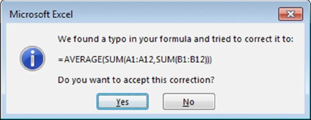
Be careful when accepting corrections for your formulas from Excel because it does not always guess correctly. For example, we entered the following formula (which has mismatched parentheses):

=AVERAGE(SUM(A1:A12,SUM(B1:B12))

Excel then proposed the following correction to the formula:

=AVERAGE(SUM(A1:A12,SUM(B1:B12)))

You may be tempted to accept the suggestion without even thinking. In this case, the proposed formula is syntactically correct—but not what we intended. The correct formula is as follows:

=AVERAGE(SUM(A1:A12),SUM(B1:B12))

Cells are filled with hash marks

A cell displays a series of hash marks (#) for one of two reasons:

§ The column is not wide enough to accommodate the formatted numeric value. To correct it, you can make the column wider or use a different number format.

§ The cell contains a formula that returns an invalid date or time. For example, Excel does not support dates prior to 1900 or the use of negative time values. Attempting to display either of these will result in a cell filled with hash marks. Widening the column won’t fix it.

Blank cells are not blank

Some Excel users have discovered that by pressing the spacebar, the contents of a cell seem to erase. Actually, pressing the spacebar inserts an invisible space character, which is not the same as erasing the cell.

For example, the following formula returns the number of nonempty cells in range A1:A10. If you “erase” any of these cells by using the spacebar, these cells are included in the count, and the formula returns an incorrect result:

=COUNTA(A1:A10)

If your formula doesn’t ignore blank cells the way that it should, check to make sure that the blank cells are really blank cells. Here’s how to search for cells that contain only a blank character:

1. Press Ctrl+F to display the Find and Replace dialog box.

2. In the Find What box, type a space character.

3. Make sure the Match Entire Cell Contents check box is selected.

4. Click Find All.

If any cells that contain only a space character are found, you’ll be able to spot them in the list displayed at the bottom of the Find and Replace dialog box.

Extra space characters

If you have formulas that rely on comparing text, be careful that your text doesn’t contain additional space characters. Adding an extra space character is particularly common when data has been imported from another source.

Excel automatically removes trailing spaces from values that you enter, but trailing spaces in text entries are not deleted. It’s impossible to tell just by looking at a cell whether text contains one or more trailing space characters.

The TRIM function removes leading spaces, trailing spaces, and multiple spaces within a text string.

Figure 22.1 shows some text in column A. The formula in B1, which was copied down the column, is

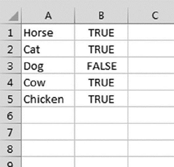
Figure 22.1 Using a formula to identify cells that contain extra space characters.

=TRIM(A1)=A1

This formula returns FALSE if the text in column A contains leading spaces, trailing spaces, or multiple spaces. In this case, the word Dog in cell A2 contains a trailing space.

Formulas returning an error

A formula may return any of the following error values:

§ #DIV/0!

§ #N/A

§ #NAME?

§ #NULL!

§ #NUM!

§ #REF!

§ #VALUE!

The following sections summarize possible problems that may cause these errors.

Tip

Excel allows you to choose the way error values are printed. To access this feature, display the Page Setup dialog box and click the Sheet tab. In the Cell Errors As drop-down, you can choose to print error values as displayed (the default) or as blank cells, dashes, or #N/A. To display the Page Setup dialog box, click the dialog box launcher in the Page Layout ➜ Page Setup group.

Tracing error values

Often, an error in one cell is the result of an error in a precedent cell (a cell that is used by the formula). To help track down the source of an error value in a cell, select the cell and choose Formulas ➜ Formula Auditing ➜ Error Checking ➜ Trace Error. Excel draws arrows to indicate the error source.

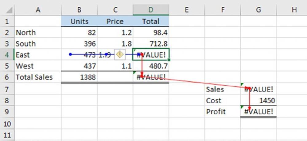
After you identify the error, use Formulas ➜ Formula Auditing ➜ Error Checking ➜ Remove Arrows to get rid of the arrow display.

#DIV/0! errors

Division by zero is not a valid operation. If you create a formula that attempts to divide by zero, Excel displays its familiar #DIV/0! error value.

Because Excel considers a blank cell to be zero, you also get this error if your formula divides by a missing value. This problem is common when you create formulas for data that you haven’t entered yet or that simply doesn’t exist, as shown in Figure 22.2. The formula in cell D2, which was copied to the cells below it, is as follows:

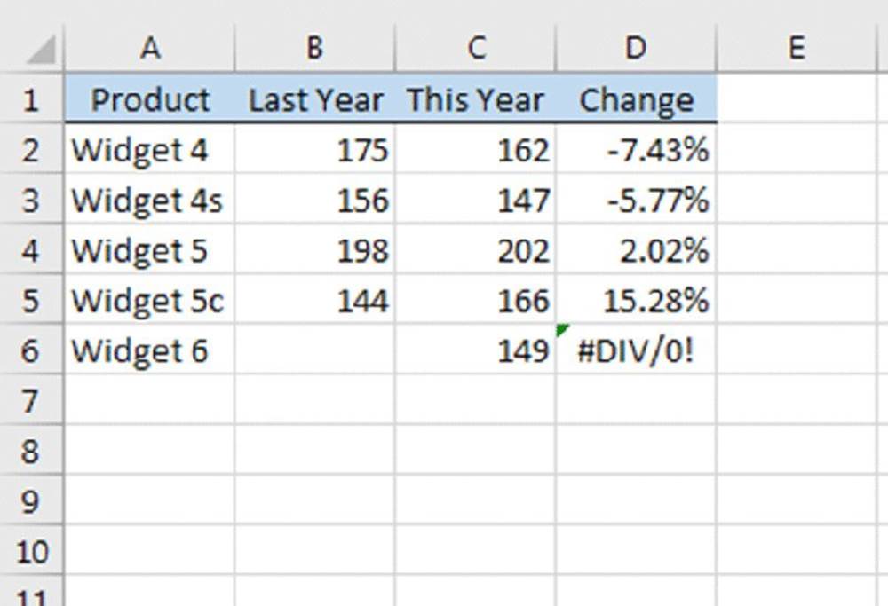
Figure 22.2 #DIV/0! errors occur when the data in column B is missing.

=(C2-B2)/B2

This formula calculates the percentage growth of a list of products from last year to this year. Because the newest product didn’t exist last year, there is no data for it, and the formula returns a #DIV/0! error.

To avoid the error display, you can use an IF function to check for a blank cell in column B:

=IF(B2=0,"", (C2-B2)/B2)

This formula displays an empty string if cell B2 is blank or contains 0; otherwise, it displays the calculated value.

Another approach is to use the IFERROR function to check for any error condition. The following formula, for example, displays an empty string if the formula results in any type of error:

=IFERROR((C2-B2)/B2,"")

IFERROR was introduced in Excel 2007. For compatibility with previous versions, use this formula:

=IF(ISERROR((C2-B2)/B2),"", (C2-B2)/B2)

#N/A errors

The #N/A error occurs if any cell referenced by a formula displays #N/A.

Note

Some users like to enter =NA() or #N/A explicitly for missing data (that is, Not Available). This method makes it perfectly clear that the data is not available and hasn’t been deleted accidentally.

The #N/A error also occurs when a lookup function (HLOOKUP, LOOKUP, MATCH, or VLOOKUP) can’t find a match.

If you would like to display an empty string instead of #N/A, use the IFNA function in a formula like this:

=IFNA(VLOOKUP(A1,C1:F50,4,FALSE),"")

Tip

The IFNA function was introduced in Excel 2013. For compatibility with previous versions, use a formula like this:

=IF(ISNA(VLOOKUP(A1,C1:F50,4,FALSE)),"",VLOOKUP(A1,C1:F50,4,FALSE))

A third common cause of #N/A errors occurs when the components of an array formula don’t contain the same number of elements. In this example, an array formula is used to find the largest value where column A is North and column B is June.

{=MAX((A1:A100="North")*(B1:B99="June")*(C1:C100))}

The first and third arrays look at 100 rows, whereas the second array only includes 99 rows. Because of this difference, this formula will return #N/A.

Cross-Ref

Array formulas are discussed in Chapter 14, “Introducing Arrays.”

#NAME? errors

The #NAME? error occurs under these conditions:

§ The formula contains an undefined range or cell name.

§ The formula contains text that Excel interprets as an undefined name. A misspelled function name, for example, generates a #NAME? error.

§ The formula contains text that isn’t enclosed in quotation marks.

§ The formula contains a range reference that omits the colon between the cell addresses.

§ The formula uses a worksheet function that’s defined in an add-in, and the add-in is not installed.

Note

Excel has a bit of a problem with range names. If you delete a name for a cell or range and the name is used in a formula, the formula continues to use the name even though it’s no longer defined. As a result, the formula displays #NAME?. You may expect Excel to automatically convert the names to their corresponding cell references, but this does not happen. In fact, Excel does not even provide a way to convert the names used in a formula to the equivalent cell references!

#NULL! errors

The #NULL! error occurs when a formula attempts to use the intersection of two ranges that don’t actually intersect. Excel’s intersection operator is a space. The following formula, for example, returns #NULL! because the two ranges have no cells in common:

=SUM(B5:B14 A16:F16)

The following formula does not return #NULL! but instead displays the contents of cell B9—which represents the intersection of the two ranges:

=SUM(B5:B14 A9:F9)

You also see a #NULL! error if you accidentally omit an operator in a formula. For example, this formula is missing the second operator:

= A1+A2 A3

#NUM! errors

A formula returns a #NUM! error if any of the following occurs:

§ You pass a nonnumeric argument to a function when a numeric argument is expected: for example, $1,000 instead of 1000.

§ You pass an invalid argument to a function. For example, this formula returns #NUM!:

=SQRT(–1)

§ A function that uses iteration can’t calculate a result. Examples of functions that use iteration are IRR and RATE.

§ A formula returns a value that is too large or too small. Excel supports values between –1E–307 and 1E+307.

#REF! errors

The #REF! error occurs when a formula uses an invalid cell reference. This error can occur in the following situations:

§ You delete a cell or the row or column of a cell that is referenced by the formula. For example, the following formula displays a #REF! error if row 1, column A, or column B is deleted:

=A1/B1

§ You delete the worksheet of a cell that is referenced by the formula. For example, the following formula displays a #REF! error if Sheet2 is deleted:

=Sheet2!A1

§ You copy a formula to a location that invalidates the relative cell references. For example, if you copy the following formula from cell A2 to cell A1, the formula returns #REF! because it attempts to refer to a nonexistent cell:

=A1–1

§ You cut a cell (by choosing Home ➜ Clipboard ➜ Cut) and then paste it to a cell that’s referenced by a formula. The formula displays #REF!.

#VALUE! errors

The #VALUE! error is common and can occur under the following conditions:

§ An argument for a function is of an incorrect data type or the formula attempts to perform an operation using incorrect data. For example, a formula that adds a value to a text string returns the #VALUE! error.

§ A function’s argument is a range when it should be a single value.

§ A custom worksheet function (created using VBA) is not calculated. With some versions of Excel, inserting or moving a sheet may cause this error. You can press Ctrl+Alt+F9 to force a recalculation.

§ A custom worksheet function attempts to perform an operation that is not valid. For example, custom functions cannot modify the Excel environment or make changes to other cells.

§ You forget to press Ctrl+Shift+Enter when entering an array formula.

Pay attention to the colors

When you edit a cell that contains a formula, Excel color-codes the cell and range references in the formula. Excel also outlines the cells and ranges used in the formula by using corresponding colors. Therefore, you can see at a glance the cells that are used in the formula.

You also can manipulate the colored outline to change the cell or range reference. To change the references that are used in the formula, drag the outline’s border or fill handle (at the lower-right corner of the outline). Using this technique is often easier than editing the formula.

Absolute/relative reference problems

As we describe in Chapter 2, “Basic Facts About Formulas,” a cell reference can be relative (for example, A1), absolute (for example, $A$1), or mixed (for example, $A1 or A$1). The type of cell reference that you use in a formula is relevant only if the formula will be copied to other cells.

A common problem is to use a relative reference when you should use an absolute reference. As shown in Figure 22.3, cell C1 contains a tax rate, which is used in the formulas in column C. The formula in cell C4 is as follows:

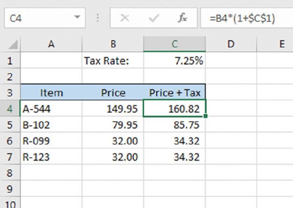
Figure 22.3 Formulas in the range C4:C7 use an absolute reference to cell C1.

=B4*(1+$C$1)

Notice that the reference to cell C1 is an absolute reference. When the formula is copied to other cells in column C, the formula continues to refer to cell C1. If the reference to cell C1 were a relative reference, the copied formulas would return an incorrect result or #VALUE!.

Operator precedence problems

Excel has some straightforward rules about the order in which mathematical operations are performed in a formula. In Table 22.1, operations with a lower precedence number are performed before operations with a higher precedence number. This table, for example, shows that multiplication has a higher precedence than addition. Therefore, multiplication is performed first.

Table 22.1: Operator Precedence in Excel Formulas

When in doubt (or when you simply need to clarify your intentions), use parentheses to ensure that operations are performed in the correct order. For example, the following formula multiplies A1 by A2 and then adds 1 to the result. The multiplication is performed first because it has a higher order of precedence.

=1+A1*A2

The following is a clearer version of this formula. The parentheses aren’t necessary—but in this case, the order of operations is perfectly obvious.

=1+(A1*A2)

Notice that the negation operator symbol is the same as the subtraction operator symbol. This, as you may expect, can cause some confusion. Consider these two formulas:

=–3^2

=0–3^2

The first formula, as expected, returns 9. The second formula, however, returns –9. Squaring a number always produces a positive result, so how is it that Excel can return the –9 result?

In the first formula, the minus sign is a negation operator and has the highest precedence. However, in the second formula, the minus sign is a subtraction operator, which has a lower precedence than the exponentiation operator. Therefore, the value 3 is squared, and the result is subtracted from zero, producing a negative result.

Note

Excel is a bit unusual in interpreting the negation operator. Other spreadsheet products (for example, Lotus 1-2-3 and Quattro Pro) return –9 for both formulas. Excel’s VBA language also returns –9 for these expressions.

Formulas are not calculated

If you use custom worksheet functions written in VBA, you may find that formulas that use these functions fail to get recalculated and may display incorrect results. For example, assume that you wrote a VBA function that returns the number format of a referenced cell. If you change the number format, the function continues to display the previous number format. That’s because changing a number format doesn’t trigger a recalculation.

To force a single formula to be recalculated, select the cell, press F2, and then press Enter. To force a recalculation of all formulas, press Ctrl+Alt+F9.

See Part VI, “Developing Custom Worksheet Functions,” for more information about creating custom worksheet functions with VBA.

Actual versus displayed values

You may encounter a situation in which values in a range don’t appear to add up properly. For example, Figure 22.4 shows a worksheet with the following formula entered into each cell in the range B3:B5:

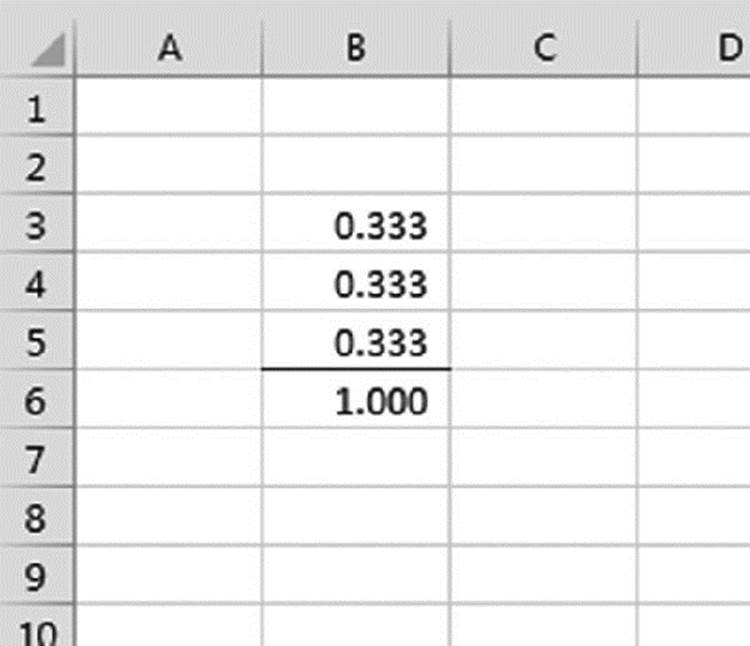
Figure 22.4 A simple demonstration of numbers that appear to add up incorrectly.

=1/3

Cell B6 contains the following formula:

=SUM(B3:B5)

All the cells are formatted to display with three decimal places. As you can see, the formula in cell B6 appears to display an incorrect result. (You may expect it to display 0.999.) The formula, of course, does return the correct result. The formula uses the actual values in the range B3:B5, not the displayed values.

You can instruct Excel to use the displayed values by selecting the Set Precision as Displayed check box on the Advanced tab of the Excel Options dialog box. (Choose File➜ Options to display this dialog box.) This setting applies to the active workbook.

Warning

Use the Set Precision as Displayed option with caution, and make sure that you understand how it works. This setting also affects normal values (nonformulas) that have been entered into cells. For example, if a cell contains the value 4.68 and is displayed with no decimal places (that is, 5), selecting the Set Precision as Displayed check box converts 4.68 to 5.00. This change is permanent, and you can’t restore the original value if you later clear the Set Precision as Displayed check box. A better approach is to use Excel’s ROUND function to round the values to the desired number of decimal places. (See Chapter 10, “Miscellaneous Calculations.”)

Floating-point number errors

Computers, by their very nature, don’t have infinite precision. Excel stores numbers in binary format by using 8 bytes, which can handle numbers with 15-digit accuracy. Some numbers can’t be expressed precisely by using 8 bytes, so the number is stored as an approximation.

To demonstrate how this limited precision may cause problems, enter the following formula into cell A1:

=(5.1–5.2)+1

The result should be 0.9. However, if you format the cell to display 15 decimal places, you’ll discover that Excel calculates the formula with a result of 0.899999999999999. This small error occurs because the operation in parentheses is performed first, and this intermediate result stores in binary format by using an approximation. The formula then adds 1 to this value, and the approximation error is propagated to the final result.

In many cases, this type of error does not present a problem. However, if you need to test the result of that formula by using a logical operator, it may present a problem. For example, the following formula (which assumes that the previous formula is in cell A1) returns FALSE:

=A1=.9

One solution to this type of error is to use Excel’s ROUND function. The following formula, for example, returns TRUE because the comparison is made by using the value in A1 rounded to one decimal place:

=ROUND(A1,1)=0.9

Here’s another example of a “precision” problem. Try entering the following formula:

=(1.333–1.233)–(1.334–1.234)

This formula should return 0, but it actually returns –2.22045E–16 (a number very close to zero).

If that formula were in cell A1, the following formula would return the string Not Zero.

=IF(A1=0,"Zero","Not Zero")

One way to handle these very-close-to-zero rounding errors is to use a formula like this:

=IF(ABS(A1)<1E–6,"Zero","Not Zero")

This formula uses the less-than operator to compare the absolute value of the number with a very small number. This formula would return Zero.

Phantom link errors

You may open a workbook and see a message like the one shown in Figure 22.5. This message sometimes appears even when a workbook contains no linked formulas.

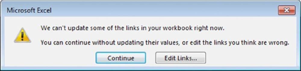
Figure 22.5 Excel’s way of asking whether you want to update links in a workbook.

First, try choosing File ➜ Info ➜ Edit Links to Files to display the Edit Links dialog box. Then select each link and click Break Link. If that doesn’t solve the problem, this phantom link may be caused by an erroneous name. Choose Formulas ➜ Defined Names ➜ Name Manager, and scroll through the list of names in the Name Manager dialog box. If you see a name that refers to #REF!, delete the name. The Name Manager dialog box has a Filter button that lets you filter the names. For example, you can filter the lists to display only the names with errors.

Cross-Ref

These phantom links may be created when you copy a worksheet that contains names. See Chapter 3, “Working with Names,” for more information about names.

Logical value errors

As you know, you can enter TRUE or FALSE into a cell to represent logical True or logical False. Although these values seem straightforward enough, Excel is inconsistent about how it treats TRUE and FALSE.

Figure 22.6 shows a worksheet with three logical values in A1:A3 as well as four formulas that sum these logical values in A5:A8. As you see, these formulas return different answers.

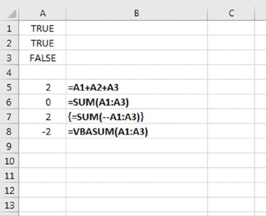
Figure 22.6 This worksheet demonstrates an inconsistency when summing logical values.

The formula in cell A5 uses the addition operator. The sum of these three cells is 2. The conclusion: Excel treats TRUE as 1 and FALSE as 0.

But wait! The formula in cell A6 uses Excel’s SUM function. In this case, the sum of these three cells is 0. In other words, the SUM function ignores logical values. However, it’s possible to force these logical values to be treated as values by the SUM function by using an array formula. The array formula in A7 uses double negation to coerce the TRUE and FALSE values to numbers.

To add to the confusion, the SUM function does return the correct answer if the logical values are passed as literal arguments. The following formula returns 2:

=SUM(TRUE,TRUE,FALSE)

Although the VBA macro language is tightly integrated with Excel, sometimes it appears that the two applications don’t understand each other. We created a simple VBA function that adds the values in a range. The function (which follows) returns –2!

Function VBASUM(rng)

Dim cell As Range

VBASUM = 0

For Each cell In rng

VBASUM = VBASUM + cell.Value

Next cell

End Function

VBA considers TRUE to be –1 and FALSE to be 0.

The conclusion is that you need to be aware of Excel’s inconsistencies and be careful when summing a range that contains logical values.

Circular reference errors

A circular reference is a formula that contains a reference to the cell that contains the formula. The reference may be direct or indirect. For help tracking down a circular reference, see the following section.

Excel’s Auditing Tools

Excel includes a number of tools that can help you track down formula errors. The following sections describe the auditing tools built into Excel.

Identifying cells of a particular type

The Go to Special dialog box is a handy tool that enables you to locate cells of a particular type. Choose Home ➜ Editing ➜ Find & Select ➜ Go to Special; see Figure 22.7.

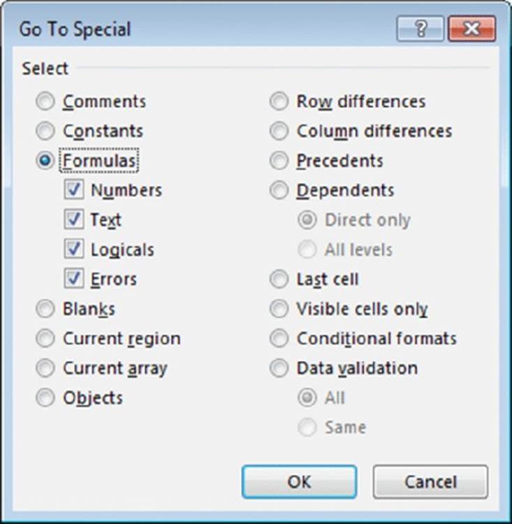
Figure 22.7 The Go to Special dialog box.

Note

If you select a multicell range before displaying the Go to Special dialog box, the command operates only within the selected cells. If a single cell is selected, the command operates on the entire worksheet.

You can use the Go to Special dialog box to select cells of a certain type, which can often help you identify errors. For example, if you choose the Formulas option, Excel selects all the cells that contain a formula. If you find a cell that’s not selected amid a group of selected formula cells, chances are good that the cell previously contained a formula that has been replaced by a value.

Viewing formulas

You can often understand an unfamiliar workbook by displaying the formulas rather than the results of the formulas. To toggle the display of formulas, choose Formulas ➜Formula Auditing ➜ Show Formulas. You may want to create a second window for the workbook before issuing this command. This way, you can see the formulas in one window and the results of the formula in the other window. Choose View ➜ Window ➜ New Window to open a new window.

Tip

You can also use Ctrl+` (the accent grave key, usually located above the Tab key) to toggle between Formula view and Normal view.

Figure 22.8 shows an example of a worksheet displayed in two windows. The window on the top shows Normal view (formula results), and the window on the bottom displays the formulas. The View ➜ Window ➜ View Side by Side command, which allows synchronized scrolling, is also useful for viewing two windows.

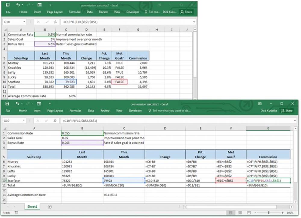
Figure 22.8 Displaying formulas (bottom window) and their results (top window).

When Formula view is in effect, Excel highlights the cells that are used by the formula in the active cell. In Figure 22.8, for example, the active cell is G10. The four cells used by this formula are highlighted in both windows.

Using the Inquire add-in

Some versions of Excel 2016 include a useful auditing add-in called Inquire. To install Inquire, choose File ➜ Options to display the Excel Options dialog box. Click the Add-Ins tab. At the bottom of the dialog box, choose COM Add-Ins from the Manage drop-down list, and click Go.

In the COM Add-Ins dialog box, place a checkmark next to Inquire Add-In and click OK. The add-in will be loaded automatically when Excel starts. If Inquire is not listed, your version of Excel does not include the add-in.

Inquire is accessible from the Inquire tab on the Ribbon. You can use this add-in to accomplish the following:

· Compare versions of a workbook

· Analyze a workbook for potential problems and inconsistencies

· Display interactive diagnostics

· Visualize links between workbook and worksheets

· Clear excess cell formatting

· Manage passwords

Tracing cell relationships

To understand how to trace cell relationships, you need to familiarize yourself with the following two concepts:

§ Cell precedents: Applicable only to cells that contain a formula; a formula cell’s precedents are all the cells that contribute to the formula’s result. A direct precedent is a cell that you use directly in the formula. An indirect precedent is a cell that is not used directly in the formula but is instead used by a cell that you refer to in the formula.

§ Cell dependents: These are formula cells that depend on a particular cell. A cell’s dependents consist of all formula cells that use the cell. Again, the formula cell can be a direct dependent or an indirect dependent.

For example, consider this simple formula entered into cell A4:

=SUM(A1:A3)

Cell A4 has three precedent cells (A1, A2, and A3), which are all direct precedents. Cells A1, A2, and A3 each have at least one dependent cell (cell A4), and A4 is a direct dependent of all of them.

Identifying cell precedents for a formula cell often sheds light on why the formula is not working correctly. Conversely, knowing which formula cells depend on a particular cell is also helpful. For example, if you’re about to delete a formula, you may want to check whether it has dependents.

Identifying precedents

You can identify cells used by a formula in the active cell in a number of ways:

§ Press F2. The cells that are used directly by the formula are outlined in color, and the color corresponds to the cell reference in the formula. This technique is limited to identifying cells on the same sheet as the formula.

§ Display the Go to Special dialog box. (Choose Home ➜ Editing ➜ Find & Select ➜ Go To Special.) Select the Precedents option and then select either Direct Only (for direct precedents only) or All Levels (for direct and indirect precedents). Click OK, and Excel selects the precedent cells for the formula. This technique is limited to identifying cells on the same sheet as the formula.

§ Press Ctrl+[ to select all direct precedent cells on the active sheet.

§ Press Ctrl+Shift+[ to select all precedent cells (direct and indirect) on the active sheet.

§ Choose Formulas ➜ Formula Auditing ➜ Trace Precedents. Excel draws arrows to indicate the cell’s precedents. Click this button multiple times to see additional levels of precedents. Choose Formulas ➜ Formula Auditing ➜ Remove Arrows to hide the arrows. Figure 22.9 shows a worksheet with precedent arrows drawn to indicate the precedents for the formula in cell C13.

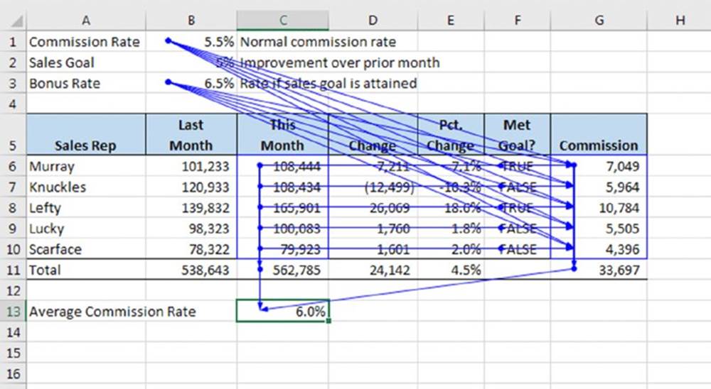
Figure 22.9 This worksheet displays lines that indicate cell precedents for the formula in cell C13.

Identifying dependents

You can identify formula cells that use a particular cell in a number of ways:

§ Display the Go to Special dialog box. Select the Dependents option and then select either Direct Only (for direct dependents only) or All Levels (for direct and indirect dependents). Click OK. Excel selects the cells that depend on the active cell. This technique is limited to identifying cells on the active sheet only.

§ Press Ctrl+] to select all direct dependent cells on the active sheet.

§ Press Ctrl+Shift+] to select all dependent cells (direct and indirect) on the active sheet.

§ Choose Formulas ➜ Formula Auditing ➜ Trace Dependents. Excel draws arrows to indicate the cell’s dependents. Click this button multiple times to see additional levels of dependents. Choose Formulas ➜ Formula Auditing ➜ Remove Arrows to hide the arrows.

Tracing error values

If a formula displays an error value, Excel can help you identify the cell that is causing that error value. An error in one cell is often the result of an error in a precedent cell. Activate a cell that contains an error value and choose Formulas ➜ Formula Auditing ➜ Error Checking ➜ Trace Error. Excel draws arrows to indicate the error source.

Fixing circular reference errors

If you accidentally create a circular reference formula, Excel displays a warning message, displays Circular Reference (with the cell address) in the status bar, and draws arrows on the worksheet to help you identify the problem.

If you can’t figure out the source of the problem, use Formulas ➜ Formula Auditing ➜ Error Checking ➜ Circular References. This command displays a list of all cells that are involved in the circular references. Start by selecting the first cell listed and then work your way down the list until you figure out the problem.

Using background error checking

Some people may find it helpful to take advantage of Excel’s automatic error-checking feature. This feature is enabled or disabled via the Enable Background Error Checking check box, on the Formulas tab of the Excel Options dialog box shown in Figure 22.10. In addition, you can specify which types of errors to check for by using the check boxes in the Error Checking Rules section.

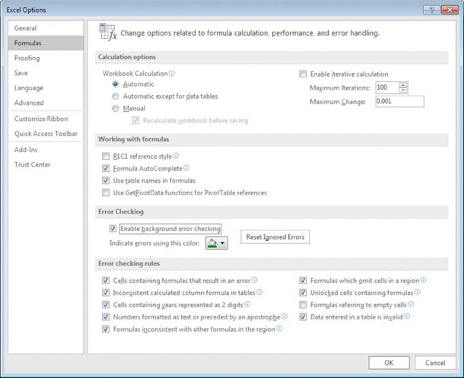
Figure 22.10 Excel can check your formulas for potential errors.

When error checking is turned on, Excel continually evaluates your worksheet, including its formulas. If a potential error is identified, Excel places a small triangle in the upper-left corner of the cell. When the cell is activated, an icon appears. Clicking this icon provides options. Figure 22.11 shows the options that appear when you click the icon in a cell that contains a #DIV/0! error. The options vary, depending on the type of error.

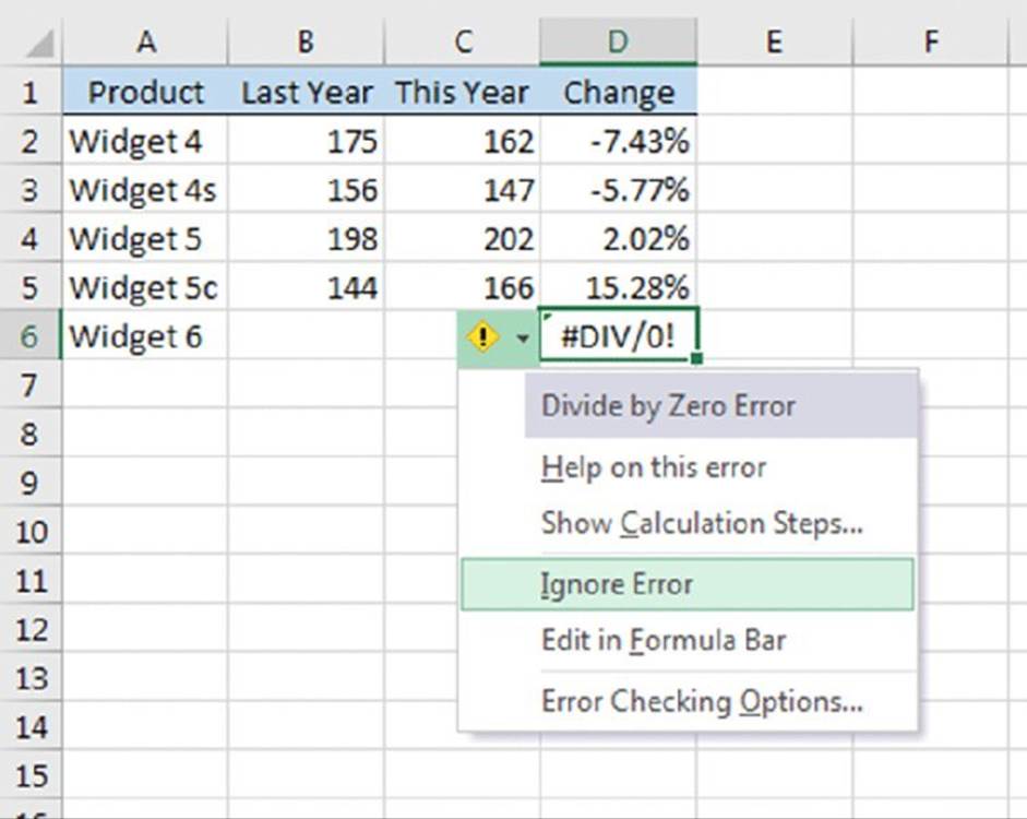
Figure 22.11 Clicking an error’s icon gives you a list of options.

In many cases, you will choose to ignore an error by selecting the Ignore Error option. Selecting this option eliminates the cell from subsequent error checks. However, all previously ignored errors can be reset so that they appear again. (Use the Reset Ignored Errors button in the Formulas tab of the Excel Options dialog box.)

You can choose Formulas ➜ Formula Auditing ➜ Error Checking to display a dialog box that describes each potential error cell in sequence, much like using a spell-checking command. This command is available even if you disable background error checking.Figure 22.12 shows the Error Checking dialog box. Note that this dialog box is modeless, so you can still access your worksheet when the Error Checking dialog box is displayed.

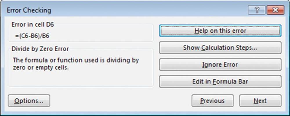
Figure 22.12 Using the Error Checking dialog box to cycle through potential errors that Excel identifies.

Warning

It’s important to understand that the error-checking feature is not perfect. In fact, it’s not even close to perfect. In other words, you can’t assume that you have an error-free worksheet simply because Excel does not identify potential errors! Also, be aware that this error checking feature won’t catch a common type of error: overwriting a formula cell with a value.

Using Excel’s Formula Evaluator

Excel’s Formula Evaluator enables you to see the various parts of a nested formula evaluated in the order that the formula is calculated.

To use the Formula Evaluator, select the cell that contains the formula and then choose Formula ➜ Formula Auditing ➜ Evaluate Formula to display the Evaluate Formula dialog box, as shown in Figure 22.13.

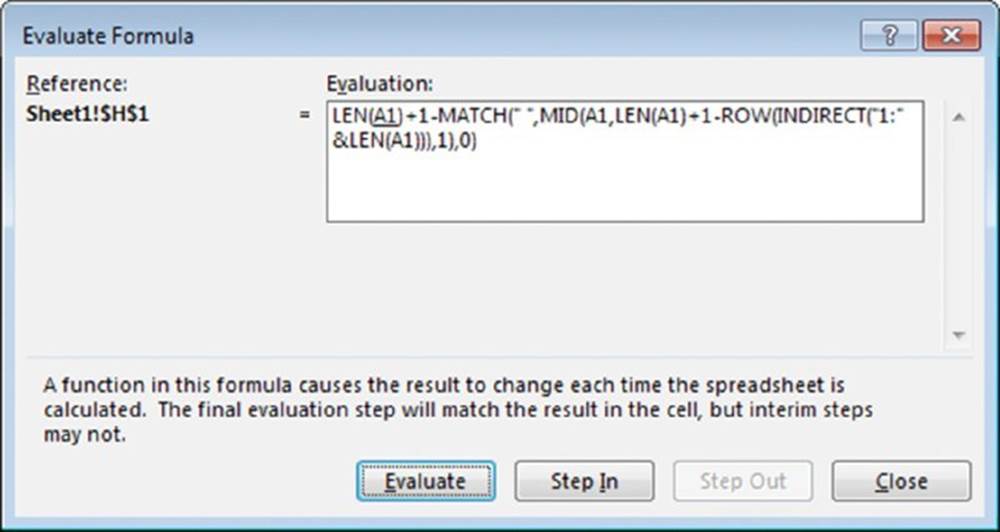
Figure 22.13 Excel’s Formula Evaluator shows a formula being calculated one step at a time.

Click the Evaluate button to show the result of calculating the expressions within the formula. Each click of the button evaluates the underlined portion of the formula. This feature may seem a bit complicated at first, but if you spend some time working with it, you’ll understand how it works and see the value.

Excel provides another way to evaluate a part of a formula:

1. Select the cell that contains the formula.

2. Press F2 to get into cell edit mode.

3. Use your mouse to highlight the portion of the formula that you want to evaluate or press Shift and use the arrow keys.

4. Press F9.

The highlighted portion of the formula displays the calculated result. You can evaluate other parts of the formula or press Esc to cancel and return your formula to its previous state.

Warning

Be careful when using this technique because if you press Enter (rather than Esc), the formula is modified to use the calculated values.