Excel 2016 Formulas (2016)

PART I
Understanding Formula Basics

Chapter 3
Working with Names

In This Chapter

· An overview and the advantages of using names in Excel

· The difference between workbook- and worksheet-level names

· Working with the Name Manager dialog box

· Shortcuts for creating cell and range names

· How to create names that extend across multiple worksheets

· How to perform common operations with range and cell names

· How Excel maintains cell and range names

· Potential problems that may crop up when you use names

· The secret behind names, and examples of named constants and named formulas

· Examples of advanced techniques that use names

Most intermediate and advanced Excel users are familiar with the concept of named cells or ranges. Naming cells and ranges is an excellent practice and offers several important advantages. As you see in this chapter, Excel supports other types of names—and the power of this concept may surprise you.

What’s in a Name?

You can think of a name as an identifier for something in a workbook. This “something” can consist of a cell, a range, a chart, a shape, and so on.

Note

Although you can give a name to any object in Excel, this chapter focuses exclusively on cell and range names (which are handled differently than other types of names).

If you provide a name for a range, you can then use that name in your formulas. For example, suppose your worksheet contains daily sales information stored in the range B2:B200. Further, assume that cell C1 contains a sales commission rate. The following formula returns the sum of the sales, multiplied by the commission rate:

=SUM(B2:B200)*C1

This formula works fine, but its purpose is not at all clear. To help clarify the formula, you can define a descriptive name for the daily sales range and another descriptive name for cell C1. Assume, for this example, that the range B2:B200 is named DailySales and cell C1 is named CommissionRate. You can then rewrite the formula to use the names instead of the actual range addresses:

=SUM(DailySales)*CommissionRate

As you can see, using names instead of cell references makes the formula self-documenting and much easier to understand.

Using named cells and ranges offers a number of advantages:

§ Names make your formulas more understandable and easier to use, especially for people who didn’t create the worksheet. Obviously, a formula such as =Income-Taxes is more intuitive than =D20-D40.

§ When entering formulas, keep in mind that a descriptive range name (such as Total_Income) is easier to remember than a cell address (such as AC21). And typing a name is less likely to result in an error than entering a cell or range address.

§ You can quickly navigate to areas of your worksheet either by using the Name box located at the left side of the Formula bar (click the arrow for a drop-down list of defined names) or by choosing Home ➜ Editing ➜ Find & Select ➜ Go To (or press F5) and specifying the range name.

§ When you select a named cell or range, its name appears in the Name box. This is a good way to verify that your names refer to the correct cells.

§ You may find that creating formulas is easier if you use named cells. You can easily insert a name into a formula by using the drop-down list that’s displayed when you enter a formula. Or press F3 to get a list of defined names.

§ Macros are easier to create and maintain when you use range names rather than cell addresses.

A Name’s Scope

Before we explain how to create and work with names, it’s important to understand that all names have a scope. A name’s scope defines where you can use the name. Names are scoped at either of two levels:

§ Workbook-level names: Can be used in any worksheet in the workbook. This is the default type of range name.

§ Worksheet-level names: Can be used only in the worksheet in which they are defined unless they are preceded with the worksheet’s name. A workbook may contain multiple worksheet-level names that are identical. For example, three sheets can have a cell named Region_Total.

Most of the time, you will use workbook-level names. For some situations, though, using worksheet-level names makes sense. For example, you might use a workbook to store monthly data, one worksheet per month. You start out with a worksheet named January, and you create worksheet-level names on that sheet. Then, rather than create a new sheet called February, you copy the January sheet and name it February. All the worksheet-level names from the January sheet are reproduced as worksheet-level names on the February sheet.

Referencing names

You can refer to a workbook-level name just by using its name from any sheet in the workbook. For worksheet-level names, you must precede the name with the name of the worksheet unless you’re using it on its own worksheet.

For example, assume that you have a workbook with two sheets: Sheet1 and Sheet2. In this workbook, you have Total_Sales (a workbook-level name), North_Sales (a worksheet-level name on Sheet1), and South_Sales (a worksheet-level name on Sheet2). On Sheet1 or Sheet2, you can refer to Total_Sales by simply using this name:

=Total_Sales

If you’re on Sheet1 and you want to refer to North_Sales, you can use a similar formula because North_Sales is defined on Sheet1:

=North_Sales

However, if you want to refer to South_Sales on Sheet1, you need to do a little more work. Sheet1 can’t “see” the name South_Sales because it’s defined on another sheet. Sheet1 can see workbook-level names and worksheet-level names only as defined on Sheet1. To refer to South_Sales on Sheet1, prefix the name with the worksheet name and an exclamation point:

=Sheet2!South_Sales

Tip

If your worksheet name contains a space, enclose the worksheet name in single quotes when referring to a name defined on that sheet:

='My Sheet'!My_Name

Note

Only the worksheet-level names on the current sheet appear in the Name box. Similarly, only worksheet-level names on the current sheet appear in the list under Formulas➜ Defined Names ➜ Use in Formulas.

Referencing names from another workbook

Chapter 2, “Basic Facts About Formulas,” describes how to use links to reference cells or ranges in other workbooks. The same rules apply when using names defined in another workbook.

For example, the following formula uses a range named MonthlySales, a workbook-level name defined in a workbook named Annual Budget.xlsx (which is assumed to be open):

=AVERAGE('Annual Budget.xlsx'!MonthlySales)

If the name MonthlySales is a worksheet-level name on Sheet1, the formula looks like this:

=AVERAGE('[Annual Budget.xlsx]Sheet1'!MonthlySales)

If you use the pointing method to create such formulas, Excel takes care of the details automatically.

Conflicting names

Using worksheet-level names can be a bit confusing because Excel lets you define worksheet-level names even if the workbook contains the same name as a workbook-level name. In such a case, the worksheet-level name takes precedence over the workbook-level name, but only in the worksheet in which you defined the sheet-level name.

For example, you can define a workbook-level name of Total for a cell on Sheet1. You can also define a worksheet-level name of Sheet2!Total. When Sheet2 is active, Total refers to the worksheet-level name. When any other sheet is active, Total refers to the workbook-level name. Confusing? Probably. To make your life easier, we recommend that you simply avoid using the same name at the workbook and worksheet levels.

One way you can avoid this type of conflict is to adopt a naming convention when you create names. By using a naming convention, your names tell you more about themselves. For instance, you can prefix all your workbook-level names with wb and your worksheet-level names with ws. With this method, you never confuse wbTotal with wsTotal.

The Name Manager

Now that you understand the concept of scope, you can start creating and using names. Excel has a handy feature for maintaining names called the Name Manager, shown in Figure 3.1.

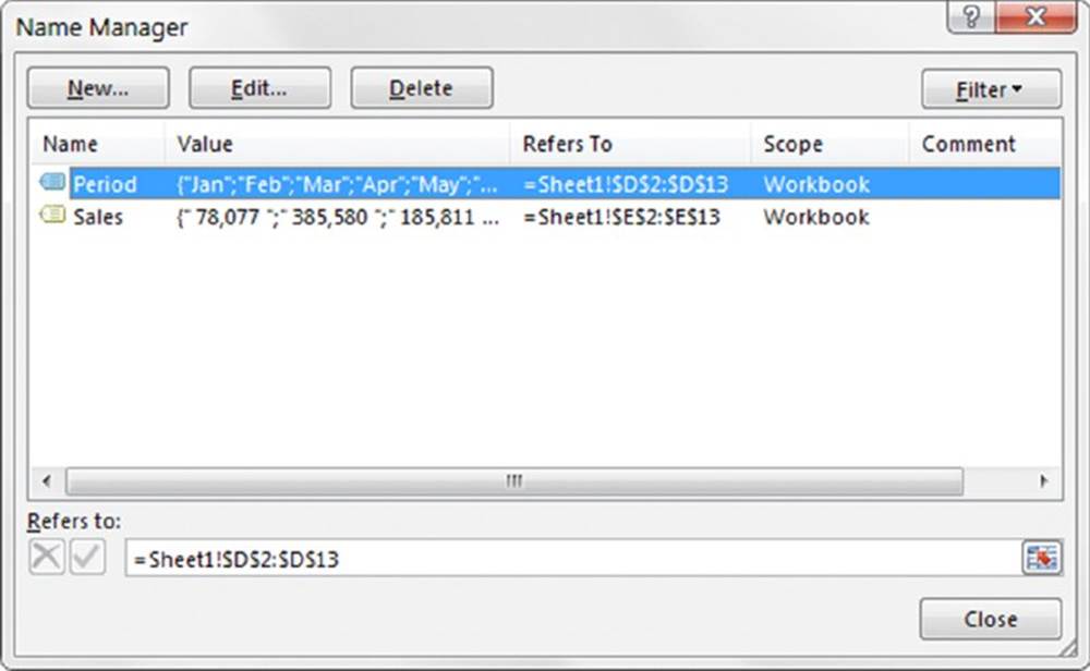
Figure 3.1 The Name Manager dialog box.

To display the Name Manager, choose Formulas ➜ Defined Names ➜ Name Manager. Within this dialog box, you can view, create, edit, and delete names. In the Name Manager main window, you can see the current value of the name, what the name refers to, the scope of the name, and any comments that you’ve written to describe the name. The names are sortable, and the columns are resizable, allowing you to see your names in many different ways. If you use a lot of names, you can also apply some predefined filters to view only the names that interest you.

Note that the Name Manager dialog box is resizable. Drag the lower-right corner to make it wider or taller.

Creating names

The Name Manager contains a New button for creating new names. The New button displays the New Name dialog box, as shown in Figure 3.2.

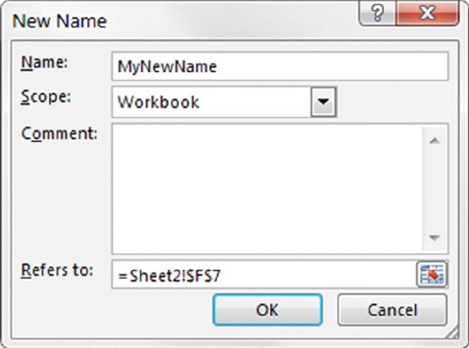
Figure 3.2 The New Name dialog box.

In the New Name dialog box, you name the name, define its scope and what it refers to, and (optionally) add any comments about the name to help yourself and others understand its purpose. The Refers To field displays the range address that was selected when you invoked the dialog box. You can change the address displayed by typing or by selecting cells in the worksheet.

Editing names

Clicking the Edit button in the Name Manager displays the Edit Name dialog box, which looks strikingly similar to the New Name dialog box. You can change any property of your name except the scope. If you change the Name field, all the formulas in your workbook that use that name are updated.

Tip

To change the scope of a name, you must delete the name and re-create it. If you’re careful to use the same name, your formulas that use that name still work.

The Edit Name dialog box isn’t the only way to edit a name. If the only property that you want to change is the Refers To property, you can do it right in the Name Manager dialog box. At the bottom of the dialog box is the field labeled Refers To. Simply select the name that you’d like to edit in the main window and change the reference in the Refers To field.

Tip

If you edit the contents of the Refers To field manually, the status bar displays Point, indicating that you’re in point mode. If you try to use keys such as the arrows, Home, or End, you find that you’re navigating around the worksheet rather than editing the Refers To text. This is a constant source of frustration to many Excel users. But there’s a simple solution. To switch from point mode to edit mode, press F2 and note that the status bar changes to show Edit.

Deleting names

Clicking the Delete button in the Name Manager permanently removes the selected name from your workbook. Excel warns you first because this action cannot be undone.

Caution

Unfortunately, Excel does not replace deleted names with the original cell references. Any formulas that use a name you delete display the #NAME? error.

Shortcuts for Creating Cell and Range Names

Excel provides a few additional ways to create names for cells and ranges other than the Name Manager. We discuss these methods in this section, along with some other relevant information that pertains to names.

The New Name dialog box

You can access the New Name dialog box directly by choosing Formulas ➜ Defined Names ➜ Define Name. The New Name dialog box that’s displayed is identical in form and function to the one from the New button on the Name Manager dialog box.

Note

A single cell or range can have any number of names. We can’t think of a good reason to use more than one name, but Excel does permit it. If a cell or range has multiple names, the Name box always displays the name that’s first alphabetically when you select the cell or range.

A name can also refer to a noncontiguous range of cells. You can select a noncontiguous range by pressing Ctrl while you select various cells or ranges with the mouse.

Rules for naming names

Although Excel is quite flexible about the names you can define, it does have some rules:

· Names can’t contain spaces. You might want to use an underscore or a period character to simulate a space (such as Annual_Total or Annual.Total).

· You can use any combination of letters and numbers, but the name must begin with a letter or underscore. A name can’t begin with a number (such as 3rdQuarter).

· A name cannot look like a cell reference. This excludes names such as Q3 and TAX2012.

· You cannot use symbols, except for underscores and periods. Although not documented, we’ve found that Excel also permits a backslash (\) and question mark (?) as long as they don’t appear as the first character in a name.

· Names cannot exceed 255 characters in length.

· You can use single letters (except for R or C). However, it is not recommended because it also defeats the purpose of using meaningful names.

· Names are not case sensitive. The name AnnualTotal is the same as annualtotal. Excel stores the name exactly as you type it when you define it, but it doesn’t matter how you capitalize the name when you use it in a formula.

Although periods are allowed, you can’t use a period if the resulting name can be construed as a range address. For example A1.A12 is not a valid name because it’s equivalent to the address A1:A12.

Excel also uses a few names internally for its own use. Although you can create names that override Excel’s internal names, you should avoid doing so unless you know what you’re doing. Generally, avoid using the following names: Print_Area, Print_Titles, Consolidate_Area, Database, Criteria, Extract, FilterDatabase, and Sheet_Title.

Creating names using the Name box

A faster way to create a name for a cell or range is to use the Name box. The Name box is the drop-down list box to the left of the Formula bar. Select the cell or range to name, click the Name box, type the name, and then press Enter to create the name. If a name already exists, you can’t use the Name box to change the range to which that name refers. Attempting to do so simply selects the original range. You must use the Name Manager dialog box to change the reference for a name.

Caution

When you type a name in the Name box, you must press Enter to actually record the name. If you type a name and then click in the worksheet, Excel doesn’t create the name.

To create a worksheet-level name using the Name box, precede the name with the active worksheet’s name, followed by an exclamation point. For example, to create the name Total as a worksheet-level name for Sheet1, type this into the Name box and press Enter:

Sheet1!Total

If the worksheet name contains spaces, enclose the sheet name in single quotes, like this:

'Summary Sheet'!Total

Because the Name box works only on the currently selected range, typing a worksheet name other than the active worksheet results in an error.

If you type an invalid name (such as May21, which is a cell address), Excel activates that address (and doesn’t warn you that the name is not valid). If the name you type includes an invalid character, Excel displays an error message.

The Name box serves double duty by also providing a quick way to activate a named cell or range. To select a named cell or range, click the Name box and choose the name, as shown in Figure 3.3. This selects the named cell or range. Oddly, the Name box does not have a keyboard shortcut. In other words, you can’t access the Name box by using the keyboard; you must use the mouse. After you click the Name box, however, you can use the direction keys and Enter to choose a name.

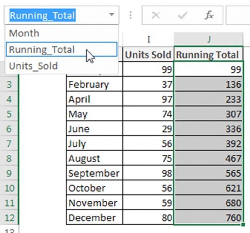
Figure 3.3 The Name box provides a quick way to select a named cell or range.

Notice that the Name box is resizable. To make the Name box wider, just click the three vertical dots icon to the right of the Name box, and drag it to the right. The Name box shares space with the Formula bar, so if you make the Name box wider, the Formula bar gets narrower.

Creating names from text in cells

You may have a worksheet containing text that you want to use for names of adjacent cells or ranges. Figure 3.4 shows an example of such a worksheet. In this case, you might want to use the text in column R to create names for the corresponding values in columns S through AD. Excel makes this easy to do.

Figure 3.4 Excel makes it easy to create names by using text in adjacent cells.

To create names by using adjacent text, start by selecting the name text and the cells that you want to name. (These can consist of individual cells or ranges of cells.) The names must be adjacent to the cells that you’re naming. (A multiple selection is allowed.) Then choose Formulas ➜ Defined Names ➜ Create from Selection (or Ctrl+Shift+F3). Excel displays the Create Names from Selection dialog box, as shown in Figure 3.5.

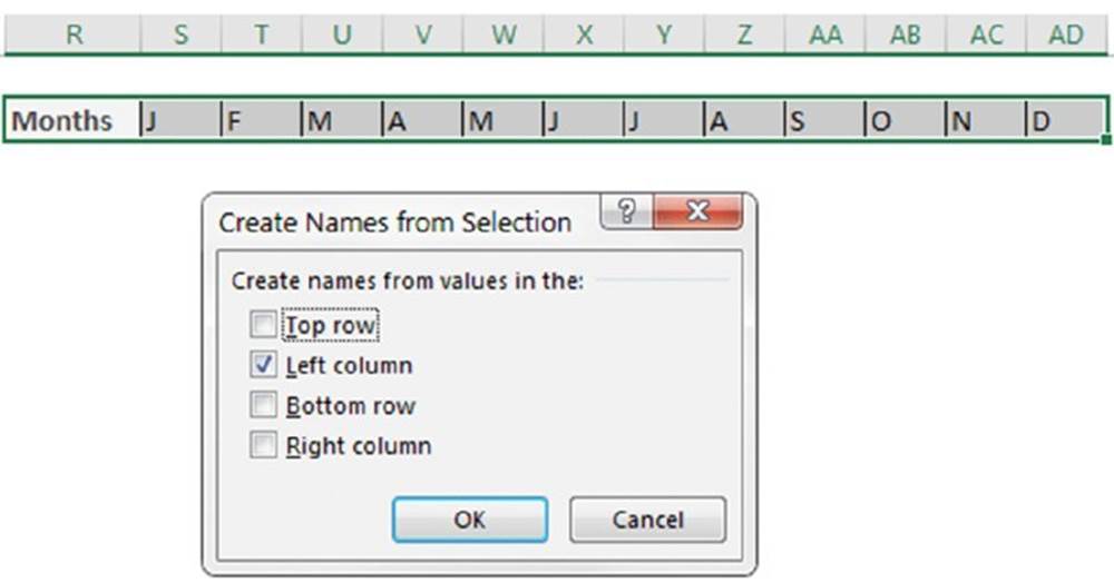
Figure 3.5 The Create Names from Selection dialog box.

The check marks in this dialog box are based on Excel’s analysis of the selected range. For example, if Excel finds text in the first row of the selection, it proposes that you create names based on the top row. If it finds text in the first column, it proposes to create names based on those cells. If Excel doesn’t guess correctly, you can change the check boxes. Click OK, and Excel creates the names.

Note that when Excel creates names using text in cells, it does not include those text cells in the named range.

If the text in a cell would result in an invalid name, Excel modifies the name to make it valid. For example, if a cell contains the text Net Income (which is invalid for a name because it contains a space), Excel converts the space to an underscore character and creates the name Net_Income. If Excel encounters a value or a formula instead of text, however, it doesn’t convert it to a valid name. It simply doesn’t create a name.

Naming entire rows and columns

Sometimes it makes sense to name an entire row or column. Often, a worksheet is used to store information that you enter over a period of time. The sheet in Figure 3.6 is an example of such a worksheet. If you create a name for the data in column I, you need to modify the name’s reference each day you add new data. The solution is to name the entire column.

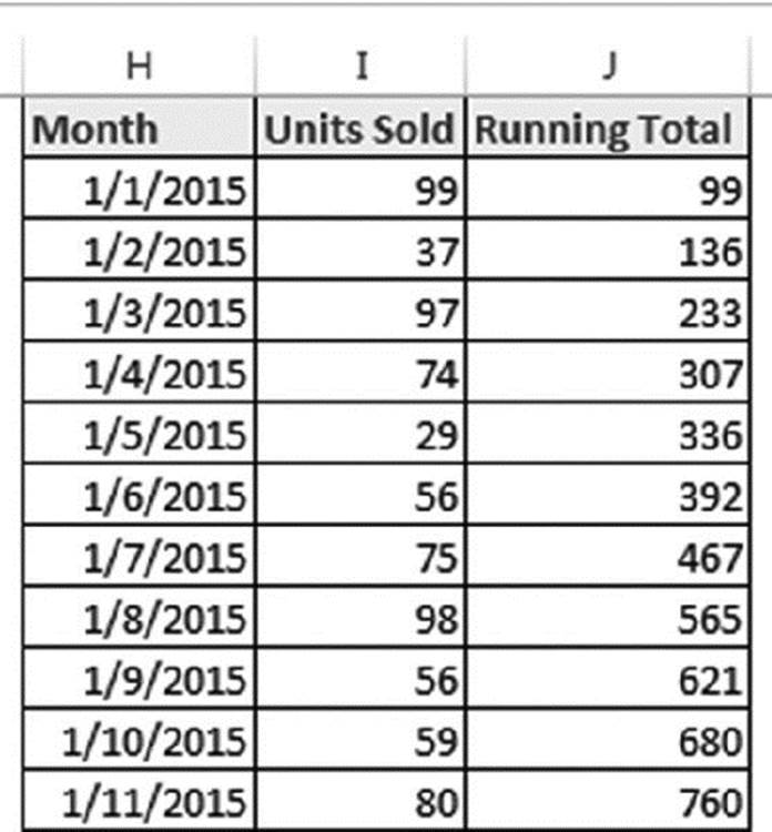
Figure 3.6 This worksheet, which tracks daily sales, uses a named range that consists of an entire column.

For example, you might name column I as DailySales. This range is on Sheet3; its reference would appear like this:

=Sheet3!$I:$I

To define a name for an entire column, select the column by clicking the column letter. Then type the name in the Name box and press Enter (or use the New Name dialog box to create the name).

After defining the name, you can use it in a formula. The following formula, for example, returns the sum of all values in column I:

=SUM(DailySales)

Names created by Excel

Excel creates some names on its own. For example, if you set a print area for a sheet, Excel creates the name Print_Area. If you set repeating rows or columns for printing, you also have a worksheet-level name called Print_Titles. When you execute a query that returns data to a worksheet, Excel assigns a name to the data that is returned. Also, many of the add-ins that ship with Excel create hidden names. (See the “Hidden names” sidebar.)

You can modify the reference for any of the names that Excel creates automatically, but make sure you understand the consequences.

Hidden names

Some Excel macros and add-ins create hidden names. These names exist in a workbook but don’t appear in the Name Manager dialog box or the Name box. For example, the Solver add-in creates a number of hidden names. Normally, you can just ignore these hidden names. However, sometimes these hidden names create problems. If you copy a sheet to another workbook, the hidden names are also copied, and they may create a link that is difficult to track down.

Although Excel’s Name Manager is versatile, it doesn’t have an option to display hidden names. Here’s a simple VBA procedure that lists all hidden names in the active workbook. The macro adds a new worksheet, and the list is written to that worksheet:

Sub ListHiddenNames()

Dim n As Name, r As Long

Worksheets.Add

r = 1

For Each n In ActiveWorkbook.Names

If Not n.Visible Then

Cells(r, 1) = n.Name

Cells(r, 2) = "'" & n.RefersTo

r = r + 1

End If

Next n

End Sub

Creating Multisheet Names

Names can extend into the third dimension; in other words, they can extend across multiple worksheets in a workbook. You can’t simply select the multisheet range and type a name in the Name box, however. You must use the New Name dialog box to create a multisheet name. The syntax for a multisheet reference is the following:

FirstSheet:LastSheet!RangeReference

In Figure 3.7, a multisheet name, DataCube, defined for A1:E5, extends across Sheet1, Sheet2, and Sheet3.

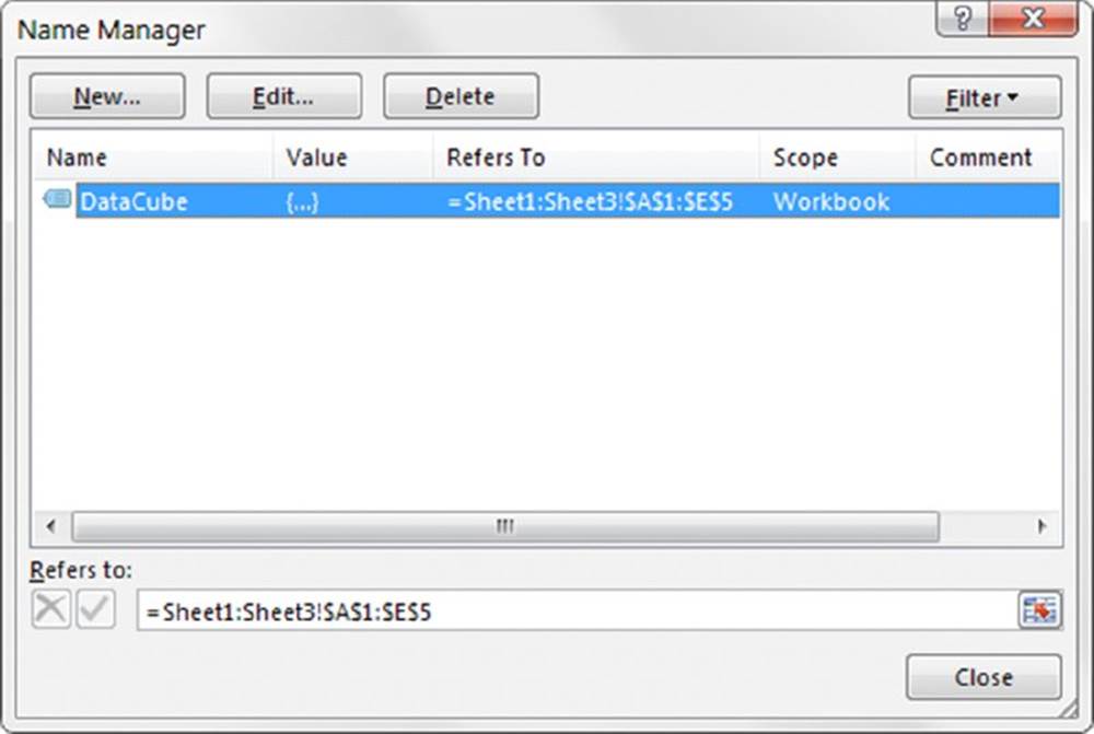
Figure 3.7 Create a multisheet name.

You can, of course, simply type the multisheet range reference in the Refers To field. If you want to create the name by pointing to the range, though, it’s a bit tricky. Even if you begin by selecting a multisheet range, Excel does not use this selected range address in the New Name dialog box.

Follow this step-by-step procedure to create a name called DataCube that refers to the range A1:E5 across three worksheets (Sheet1, Sheet2, and Sheet3):

1. Activate Sheet1.

2. Choose Formulas ➜ Defined Names ➜ Define Name to display the New Name dialog box.

3. Type DataCube into the Name field.

4. Highlight the range reference in the Refers To field and press Delete to delete the range reference.

5. Click the sheet tab for Sheet1.

6. Press Shift and click the sheet tab for Sheet3.

At this point, the Refers To field contains the following:

='Sheet1!Sheet3'!

7. Select the range A1:E5 in Sheet1 (which is still the active sheet).

The following appears in the Refers To field:

='Sheet1:Sheet3'!$A$1:$E$5

8. Because the Refers To field now has the correct multisheet range address, click OK to close the New Name dialog box.

After you define the name, you can use it in your formulas. For example, the following formula returns the sum of the values in the range named DataCube:

=SUM(DataCube)

Note

Multisheet names do not appear in the Name box or in the Go To dialog box (which appears when you choose Home ➜ Editing ➜ Find & Select & Go To). In other words, Excel enables you to define the name, but it doesn’t give you a way to automatically select the cells to which the name refers. However, multisheet names do appear in the Formula AutoComplete drop-down list that appears when you type a formula.

If you insert a new worksheet into a workbook that uses multisheet names, the multisheet names include the new worksheet—as long as the sheet resides between the first and last sheet in the name’s definition. In the preceding example, a worksheet inserted between Sheet1 and Sheet2 is included in the DataCube range. However, a worksheet inserted before Sheet1 or after Sheet3 is not included.

If you delete the first or the last sheet included in a multisheet name, Excel changes the name’s range in the Refers To field automatically. In the preceding example, deleting Sheet1 causes the Refers To range of DataCube to change to this:

='Sheet2:Sheet3'!$A$1:$E$5

Multisheet names can be scoped at the workbook level or worksheet level. If it’s a worksheet-level name, the name is valid only on the sheet that it’s scoped to.

Working with Range and Cell Names

After you create range or cell names, you can work with them in a variety of ways. This section describes how to perform common operations with range and cell names.

Creating a list of names

If you create a large number of names, you may need to know the ranges that each name refers to, particularly if you’re trying to track down errors or document your work. You might want to create a list of all names (and their corresponding addresses) in the workbook. The Name Manager dialog box doesn’t provide this option, but there’s a way to do it.

To create a list of names, first move the cell pointer to an empty area of your worksheet. (The two-column name list, created at the active cell position, overwrites any information at that location.) Use the Formulas ➜ Defined Names ➜ Use in Formula ➜ Paste Names command (or press F3). Excel displays the Paste Name dialog box that lists all the defined names. To paste a list of names, click the Paste List button. Figure 3.8 shows the Paste Name dialog box.

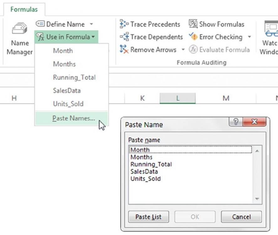
Figure 3.8 Use the Paste Name dialog box to create a list of names.

Caution

The list of names does not include hidden names or worksheet-level names that appear in sheets other than the active sheet.

The list of names pasted to your worksheet occupies two columns. The first column contains the names, and the second column contains the corresponding range addresses. The range addresses in the second column consist of text strings that look like formulas. You can convert such a string to an actual formula by editing the cell. Press F2 and then press Enter. The string then converts to a formula. If the name refers to a single cell, the formula displays the cell’s current value. If the name refers to a range, the formula may return a #VALUE! error, or, in the case of multisheet names, a #REF! error.

Cross-Ref

We discuss formula errors such as #VALUE! and #REF! in Chapter 22, “Tools and Methods for Debugging Formulas.”

Using names in formulas

After you define a name for a cell or range, you can use it in a formula. For example, the following formula calculates the sum of the values in the range named UnitsSold:

=SUM(UnitsSold)

Recall from the earlier section on scope (“A Name’s Scope”) that when you write a formula that uses a worksheet-level name on the sheet in which it’s defined, you don’t need to include the worksheet name in the range name. If you use the name in a formula on a different worksheet, however, you must use the entire name (sheet name, exclamation point, and name). For example, if the name UnitsSold represents a worksheet-level name defined on Sheet1, the following formula (on a sheet other than Sheet1) calculates the total of the UnitsSold range:

=SUM(Sheet1!UnitsSold)

When you’re composing a formula and you need to insert a name, you have three options:

§ Start typing the name, and it appears in the Formula AutoComplete drop-down list, along with a list of worksheet functions. To use Formula AutoComplete, begin typing the defined name until it is highlighted on the list, and then press Tab to complete the entry. Or use the down arrow key and press Tab to select a name from the list.

§ Press F3 to display the Paste Name dialog box. This dialog box displays a list of defined names. Just select the name and click OK, and it’s inserted into your formula.

§ Choose Formulas ➜ Defined Names ➜ Use in Formula. This command also displays a list of defined names. Click a name, and it’s inserted into your formula.

If you use a nonexistent name (or a name that’s scoped to a different worksheet) in a formula, Excel displays a #NAME? error, indicating that it cannot find the name you are trying to use. Often, this means that you misspelled the name or that the name was deleted.

Using the intersection operators with names

Excel’s range intersection operator is a single space character. The following formula, for example, displays the sum of the cells at the intersection of two ranges: B1:C20 and A8:D8:

=SUM(B1:C20 A8:D8)

The intersection of these two ranges consists of two cells: B8 and C8.

The intersection operator also works with named ranges. Figure 3.9 shows a worksheet containing named ranges that correspond to the row and column labels. For example, January refers to B2:E2, and Region3 refers to D2:D13. The following formula returns the contents of the cell at the intersection of the January range and the Region3 range:

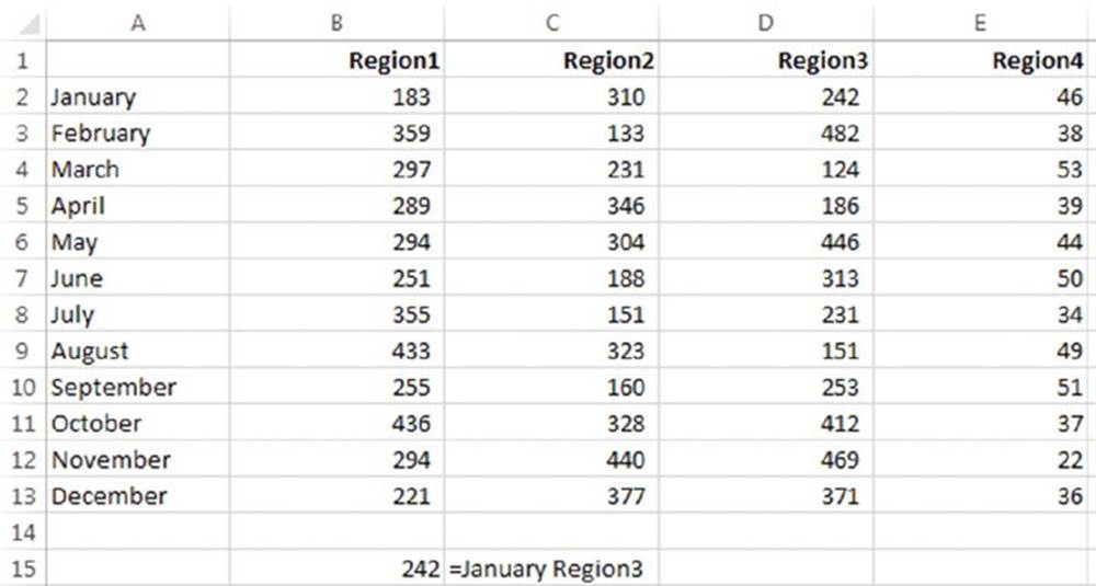
Figure 3.9 The formula in cell B15 uses the intersection operator.

=January Region3

Using a space character to separate two range references or names is known as explicit intersection because you explicitly tell Excel to determine the intersection of the ranges.

Excel can also perform implicit intersections, which occur when Excel chooses a value from a multicell range based on the row or column of the formula that contains the reference. An example should clear this up. Figure 3.10 shows a worksheet that contains a range (A2:A13) named MonthNames. Cell G5 contains the simple formula shown here:

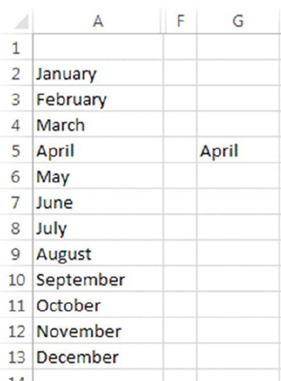
Figure 3.10 Range A2:A13 in this worksheet is named MonthNames. Cell G5 demonstrates an implicit intersection.

=MonthNames

Notice that cell G5 displays the value from MonthNames that corresponds to the formula’s row. Similarly, if you enter the same formula into any other cell in rows 3 through 14, the formula displays the corresponding value from MonthNames. Excel performs an implicit intersection using the MonthNames range and the row that contains the formula.

If you enter the formula into a cell that’s in a row not occupied by MonthNames, the formula returns an error because the implicit intersection returns nothing.

By the way, implicit intersections are not limited to named ranges. In the preceding example, you get the same result if cell G5 contains the following formula (which doesn’t use a named range):

=$A$2:$A$13

If you use MonthNames as an argument for a function, implicit intersection applies only if the function argument is interpreted as a single value. For example, if you enter this formula into cell G5, implicit intersection works, and the formula returns 5 (the number of characters in April):

=LEN(MonthNames)

But if you enter this formula, implicit intersection does not apply, and the formula returns 12, the number of cells in the MonthNames range:

=COUNTA(MonthNames)

Using the range operator with names

You can also use the range operator, which is a colon (:), to work with named ranges. Refer to Figure 3.9. For example, this formula returns the sum of the values in the 12-cell range that extends from Region1 January (cell B2) through Region4 March (cell E4):

=SUM((Region1 January):(Region4 March))

Referencing a single cell in a multicell named range

You can use Excel’s INDEX function to return a single cell from a multicell named range. Assume that range A1:A10 is named DataRange. The following formula displays the fourth value (the value in A4) in DataRange:

=INDEX(DataRange,4)

The second and third arguments for the INDEX function are optional—although at least one of them must always be specified. The second argument (used in the preceding formula) specifies the row offset within the DataRange range.

If DataRange consists of multiple cells in a single row (for example, A1:J1), use a formula like the following one to return the fourth element in the range. This formula omits the second argument for the INDEX function but uses the third argument that specifies the column offset with the DataRange range:

=INDEX(DataRange,,4)

If the range consists of multiple rows and columns, use both the second and the third arguments for the INDEX function. For example, if DataRange is defined as A1:J10, this formula returns the value in the fourth row and fifth column of the named range:

=INDEX(DataRange,4,5)

Applying names to existing formulas

When you create a name for a cell or range, Excel does not scan your formulas automatically and replace the cell references with your new name. You can, however, tell Excel to “apply” names to a range of formulas.

Select the range that contains the formulas you want to modify so they will use names rather than cell references. Then choose Formulas ➜ Defined Names ➜ Define Name➜ Apply Names. The Apply Names dialog box appears, as shown in Figure 3.11. In the Apply Names dialog box, select which names you want applied to the formulas. Only those names you select are applied to the formulas.

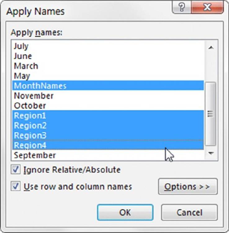
Figure 3.11 The Apply Names dialog box.

Tip

To apply names to all the formulas in the worksheet, select a single cell before you display the Apply Names dialog box.

The Ignore Relative/Absolute check box controls how Excel substitutes the range name for the actual address. A cell or range name is usually defined as an absolute reference. If the Ignore Relative/Absolute check box is selected, Excel applies the name only if the reference in the formula matches exactly. In most cases, you will want Excel to apply names whether the formulas are a relative or absolute reference. So leave the Ignore Relative/Absolute check box selected.

If the Use Row and Column Names check box is selected, Excel takes advantage of the intersection operator when applying names. Excel uses the names of row and column ranges that refer to the cells if it cannot find the exact names for the cells. Excel uses the intersection operator to join the names. Clicking the Options button displays some additional options that are available only when you select the Use Row and Column Names check box.

Applying names automatically when creating a formula

When you insert a cell or range reference into a formula by pointing, Excel automatically substitutes the cell or range name if it has one.

In some cases, this feature can be useful. In other cases, it can be annoying; you may prefer to use an actual cell or range reference instead of the name. For example, if you plan to copy the formula, the range references don’t adjust if the reference is a name rather than an address. Unfortunately, you cannot turn off this feature. If you prefer to use a regular cell or range address, you need to type the cell or range reference manually. (Don’t use the pointing technique.)

Unapplying names

Excel does not provide a direct method for unapplying names. In other words, you cannot replace a name in a formula with the name’s actual cell reference automatically. However, you can take advantage of a trick described here (which works only for workbook-level names). You need to (temporarily) change Excel’s Transition Formula Entry option so that it emulates Lotus 1-2-3.

1. Choose File ➜ Options and then click the Advanced tab in the Excel Options dialog box.

2. Under the Lotus Compatibility Settings section, place a check mark next to Transition Formula Entry and then click OK.

3. Select a cell that contains a formula that uses one or more cell or range names.

4. Press F2 and then press Enter.

5. In other words, edit the cell but don’t change anything.

6. Repeat steps 3 and 4 for other cells that use range names.

7. Go back to the Options dialog box and remove the check mark from the Transition Formula Entry check box.

The edited cells use relative range references rather than names.

Note

This trick is not documented, and it might not work in all cases, so make sure that you check the results carefully.

Names with errors

If you delete the rows or columns that contain named cells or ranges, the names are not deleted (as you might expect). Rather, each name contains an invalid reference. For example, if cell A1 on Sheet1 is named Interest and you delete row 1 or column A, Interestthen refers to =Sheet1!#REF! (that is, an erroneous reference). If you use Interest in a formula, the formula displays #REF.

To get rid of this erroneous name, you must delete the name manually using the Delete button in the Name Manager dialog box. Or you can redefine the name so it refers to a valid cell or range.

Tip

The Name Manager allows you to filter the names that it displays using predefined filters. One of the filters provided, Names with Errors, shows only those names that contain errors, which enables you to quickly locate problematic names.

Viewing named ranges

As you probably know, you can change the zoom factor of a worksheet by using the slider on the right side of the status bar (or, use commands in the View ➜ Zoom group). When you zoom a worksheet to 39 percent or smaller, you see a border around the named ranges with the name displayed in blue letters, as shown in Figure 3.12. The border and name do not print; they simply help you visualize the named ranges on your sheet.

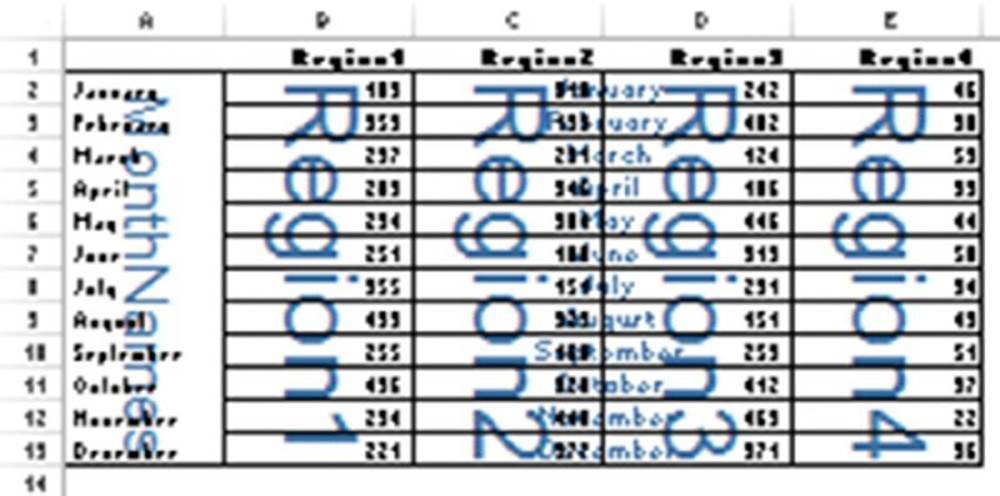
Figure 3.12 Excel displays range names when you zoom a sheet to 39 percent or less.

Using names in charts

When you create a chart, each data series has an associated SERIES formula. The SERIES formula contains references to the ranges used in the chart. If you have a defined range name, you can edit a chart’s SERIES formula and replace the range reference with the name. After doing so, the chart series adjusts if you change the definition for the name.

Cross-Ref

See Chapter 17, “Charting Techniques,” for additional information about charts.

How Excel Maintains Cell and Range Names

After you create a name for a cell or range, Excel automatically maintains the name as you edit or modify the worksheet. The following examples assume that Sheet1 contains a workbook-level name (MyRange) that refers to the following nine-cell range:

=Sheet1!$C$3:$E$5

Inserting a row or column

When you insert a row above the named range or insert a column to the left of the named range, Excel changes the range reference to reflect its new address. For example, if you insert a new row 1, MyRange then refers to =Sheet1!$C$4:$E$6.

If you insert a new row or column within the named range, the named range expands to include the new row or column. For example, if you insert a new column to the left of column E, MyRange then refers to =Sheet1!$C$3:$F$5.

Deleting a row or a column

When you delete a row above the named range or delete a column to the left of the named range, Excel adjusts the range reference to reflect its new address. For example, if you delete row 1, MyRange refers to =Sheet1!$C$2:$E$4.

If you delete a row or a column within the named range, the named range adjusts accordingly. For example, if you delete column D, MyRange then refers to =Sheet1!$C$3:$D$5.

If you delete all rows or all columns that make up a named range, the named range continues to exist, but it contains an error reference. For example, if you delete columns C, D, and E, MyRange then refers to =Sheet1!#REF!. Any formulas that use the name also return errors.

Cutting and pasting

When you cut and paste an entire named range, Excel changes the reference accordingly. For example, if you move MyRange to a new location beginning at cell A1, MyRange then refers to =Sheet1!$A$1:$C$3. Cutting and pasting only a part of a named range does not affect the name’s reference.

Potential Problems with Names

Names are great, but they can also cause some problems. This section contains information that you should remember when you use names in a workbook.

Name problems when copying sheets

Excel lets you copy a worksheet within the same workbook or to a different workbook. Focus first on copying a sheet within the same workbook. If the copied sheet contains worksheet-level names, those names are also present on the copy of the sheet, adjusted to use the new sheet name. Usually, this is exactly what you want to happen. However, if the workbook contains a workbook-level name that refers to a cell or range on the sheet that’s copied, that name is also present on the copied sheet. However, it is converted to a worksheet-level name. That is usually not what you want to happen.

Consider a workbook that contains one sheet (Sheet1). This workbook has a workbook-level name (BookLevel) for cell A1 and a worksheet-level name (Sheet1!SheetLevel) for cell A2. If you make a copy of Sheet1 within the workbook, the new sheet is named Sheet1 (2). After copying the sheet, the workbook contains four names. The new sheet has two worksheet-level names.

Not only is this proliferation of names when copying a sheet confusing, but it can result in errors that can be difficult to identify. In this case, typing the following formula on the copied sheet displays the contents of cell A1 in the copied sheet:

=BookLevel

In other words, the newly created worksheet-level name (not the original workbook-level name) is being used. This is probably not what you want.

If you copy the worksheet from a workbook containing a name that refers to a multisheet range, you also copy this name. A #REF! error appears in its Refers To field.

When you copy a sheet to a new workbook, all the names in the original workbook that refer to cells on the copied sheet are also copied to the new workbook. These include both workbook-level and worksheet-level names.

Note

Copying and pasting cells from one sheet to another does not copy names, even if the copied range contains named cells.

Bottom line? You must use caution when copying sheets from a workbook that uses names. After copying the sheet, check the names and delete those that you didn’t intend to copy.

Name problems when deleting sheets

When you delete a worksheet that contains cells used in a workbook-level name, the name is not deleted. The name remains with the workbook, but it contains an erroneous reference in its Refers To definition.

For instance, imagine your workbook contained a sheet named Sheet2, which has a workbook-level name (MyRange). After deleting Sheet2, the name MyRange still exists in the workbook, but the Refers To column displays a #Ref error for the sheet name. You might see something like this:

=#REF!$A$1:$E$12

Keeping erroneous names in a workbook doesn’t cause harm, but it’s still good practice to delete or correct all names that contain an erroneous reference.

Naming objects

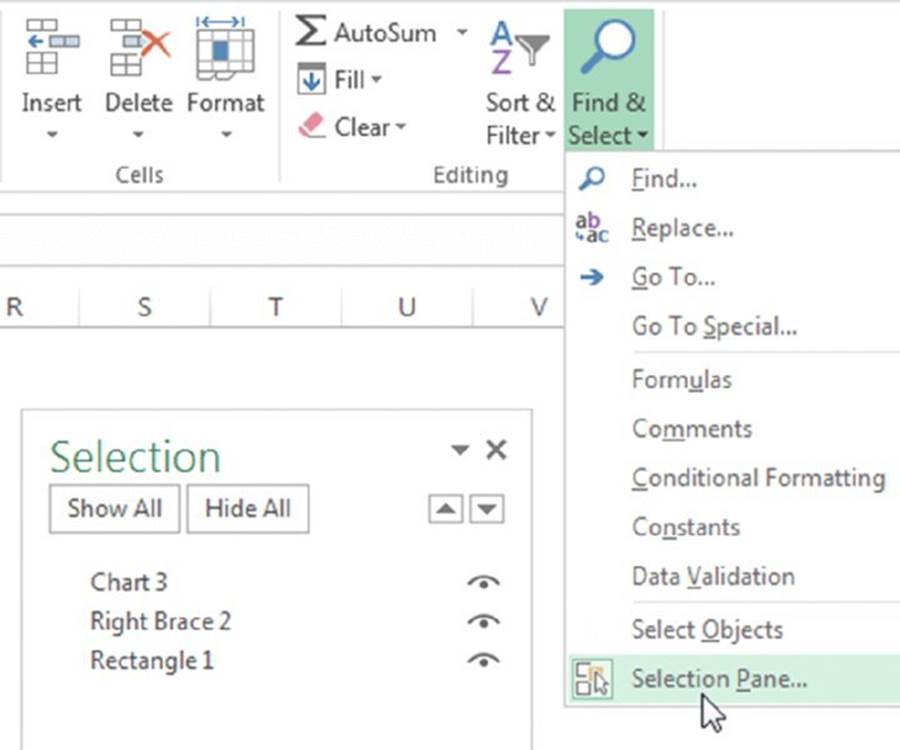
When you add an object to a worksheet (such as a shape, an image, or a chart), the object has a default name that reflects the type of object (for example, Rectangle 3 or Text Box 1).

To change the name of an object, select it, type the new name in the Name box, and press Enter.

Excel is a bit inconsistent with regard to the Name box. Although you can use the Name box to rename an object, the Name box does not display a list of objects, so you can’t use the Name box to select an object. However, you can use the Selection Pane to list all objects and make them easy to select. To display the Selection Pane, choose Home ➜ Editing ➜ Find & Select ➜ Selection Pane.

Excel also allows you to define a name with the same name as an object; two or more objects can even have the same name. The Name Manager dialog box does not list the names of objects.

The Secret to Understanding Names

Excel users often refer to named ranges and named cells. In fact, we use these terms frequently throughout this chapter. Technically, this terminology is not quite accurate.

Here’s the secret to understanding names: when you create a name, you’re actually creating a named formula. Unlike a normal formula, a named formula doesn’t exist in a cell. Rather, it exists in Excel’s memory.

This is not exactly an earth-shaking revelation, but keeping this “secret” in mind can help you understand the advanced naming techniques that follow.

When you work with the Name Manager dialog box, the Refers To field contains the formula, and the Name field contains the formula’s name. The content of the Refers To field always begins with an equal sign, which makes it a formula.

For example, if your workbook contains a name (InterestRate) referring to cell B1, that name is technically a named formula, not a named cell. Whenever you use the name InterestRate, Excel actually evaluates the formula with that name and returns the result. For example, you might type this formula into a cell:

=InterestRate*1.05

When Excel evaluates this formula, it first evaluates the formula named InterestRate (which exists only in memory, not in a cell). It then multiplies the result of this named formula by 1.05 and displays the result. This cell formula, of course, is equivalent to the following formula, which uses the actual cell reference instead of the name:

=Sheet1!$B$1*1.05

At this point, you may be wondering whether it’s possible to create a named formula that doesn’t contain cell references. The answer comes in the next section.

Naming constants

Consider a worksheet that generates an invoice and calculates sales tax for a sales amount. The common approach is to insert the sales tax rate value into a cell and then use this cell reference in your formulas. To make things easier, you probably would name this cell something like SalesTax.

You can handle this situation another way. Figure 3.13 demonstrates the following steps:

1. Choose Formulas ➜ Defined Names ➜ Define Name to bring up the New Name dialog box.

2. Type the name (in this case, SalesTax) into the Name field.

3. Click in the Refers To field, delete its contents, and replace it with a simple formula, such as =.075.

4. Click OK to close the New Name dialog box.

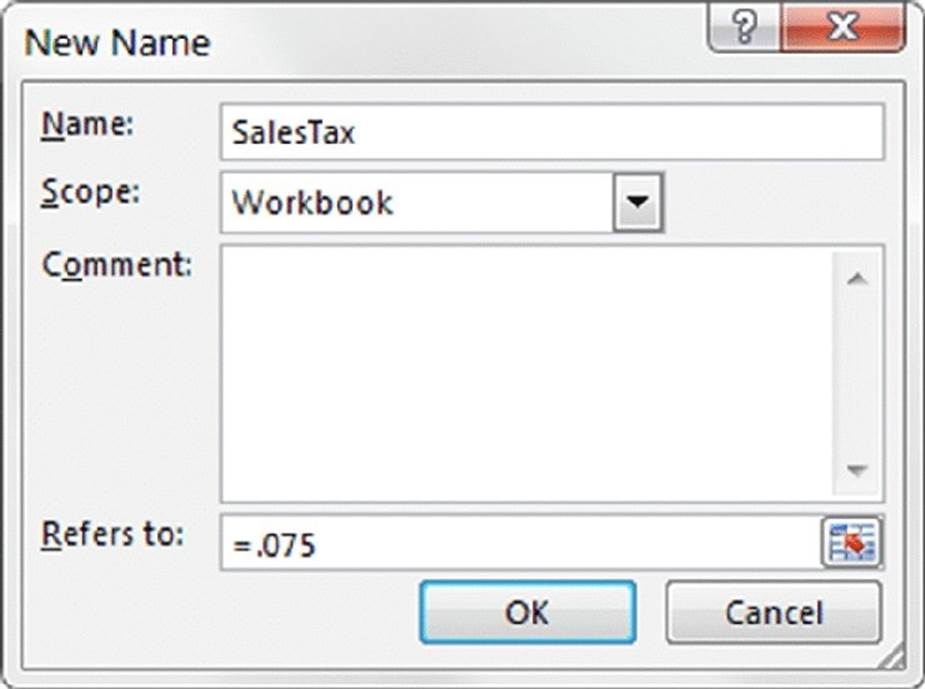
Figure 3.13 Defining a name that refers to a constant.

The preceding steps create a named formula that doesn’t use cell references. To try it out, enter the following formula into any cell:

=SalesTax

This simple formula returns .075, the result of the formula named SalesTax. Because this named formula always returns the same result, you can think of it as a named constant. And you can use this constant in a more complex formula, such as the following:

=A1*SalesTax

If you didn’t change the scope from the default of Workbook, you can use SalesTax in any worksheet in the workbook.

Naming text constants

In the preceding example, the constant consisted of a numeric value. A constant can also consist of text. For example, you can define a constant for a company’s name. You can use the New Name dialog box to create the following formula named MS:

="Microsoft Corporation"

Then you can use a cell formula, such as the following:

="Annual Report: "&MS

This formula returns the text Annual Report: Microsoft Corporation.

Note

Names that do not refer to ranges do not appear in the Name box or in the Go To dialog box (which appears when you press F5). This makes sense because these constants don’t reside anywhere tangible. They do appear in the Paste Names dialog box and in the Formula AutoComplete drop-down list, however, which makes sense because you use these names in formulas.

As you might expect, you can change the value of the constant at any time by accessing the Name Manager dialog box and changing the formula in the Refers To field. When you close the dialog box, Excel uses the new value to recalculate the formulas that use this name.

Although this technique is useful in many situations, changing the value takes some time. Having a constant located in a cell makes it much easier to modify.

Using worksheet functions in named formulas

Figure 3.14 shows another example of a named formula. In this case, the formula is named ThisMonth, and the actual formula is this:

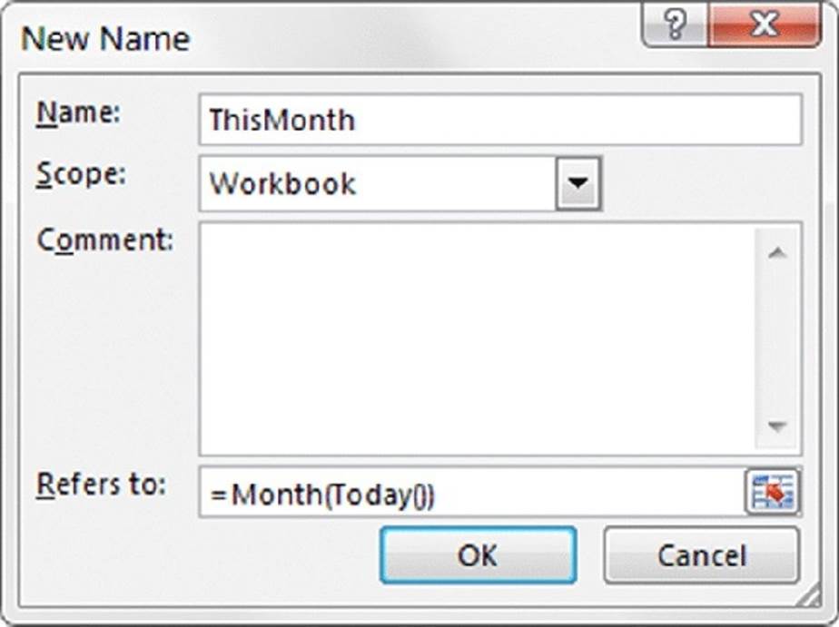
Figure 3.14 Defining a named formula that uses worksheet functions.

=MONTH(TODAY())

The formula in Figure 3.14 uses two worksheet functions. The TODAY function returns the current date, and the MONTH function returns the month number of its date argument. Therefore, you can enter a formula such as the following into a cell, and it returns the number of the current month. For example, if the current month is April, the formula returns 4:

=ThisMonth

A more useful named formula would return the actual month name as text. To do so, create a formula named MonthName, defined as follows:

=TEXT(TODAY(),"mmmm")

Cross-Ref

See Chapter 5, “Manipulating Text,” for more information about Excel’s TEXT function.

Now enter the following formula into a cell, and it returns the current month name as text. In the month of April, the formula returns the text April:

=MonthName

Using cell and range references in named formulas

Figure 3.15 shows yet another example of creating a named formula, this time with a cell reference. This formula, named FirstChar, returns the first character of the contents of cell A1 on Sheet1. This formula uses the LEFT function, which returns characters from the left part of a text string. The named formula is the following:

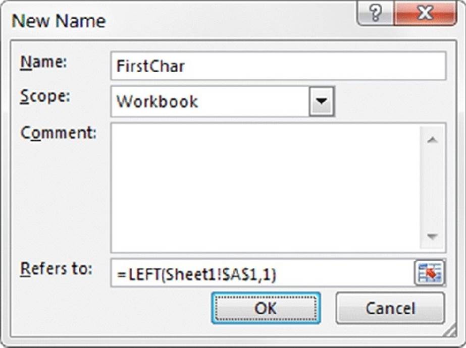
Figure 3.15 Defining a named formula that uses a cell reference.

=LEFT(Sheet1!$A$1,1)

After creating this named formula, you can enter the following formula into a cell. The formula always returns the first character of cell A1 on Sheet1:

=FirstChar

Note that if you insert a new row above row 1, the reference in the FirstChar name adjusts so it shows the first character in cell A2. It’s possible to create a name that always refers to a specific cell or range, even if you insert new rows or columns. For example, suppose you want the name FirstChar to always refer to cell A1. You need to modify the formula for FirstChar so that it users the INDIRECT function:

=LEFT(INDIRECT("$A$1"),1)

After creating this named formula, FirstChar always returns the first character in cell A1, even if you insert new rows or columns. The INDIRECT function, in the preceding formula, lets you specify a cell address indirectly by using a text argument. Because the argument appears in quotation marks, it never changes.

Here’s an example that uses a range reference in a named formula. The formula named ColumnACount returns the number of nonempty cells in column A of Sheet1. The formula is this:

=COUNTA(Sheet1!$A:$A)

You can display this count in a cell by using this formula:

=ColumnACount

Note, however, that entering this formula in column A of Sheet1 results in a circular reference error—just what you would expect.

Notice that the cell references in the preceding named formulas are absolute references. By default, all cell and range references in named formulas use an absolute reference, with the worksheet qualifier. But, as you can see in the next section, overriding this default behavior by using a relative cell reference can result in some interesting named formulas.

Using named formulas with relative references

As we noted previously, when you use the New Name dialog box to create a named formula that refers to cells or ranges, the Refers To field always uses absolute cell references, and the references include the sheet name qualifier. In this section, we describe how to use relative cell and range references in named formulas.

Using a relative cell reference

Begin by following these steps to create a named formula that uses a relative reference:

1. Start with an empty worksheet.

2. Select cell A1.

This step is important.

3. Choose Formulas ➜ Defined Names ➜ Define Name.

This brings up the New Name dialog box.

4. Type CellToRight in the Name field.

5. Delete the contents of the Refers To field and type the following formula. (Don’t point to the cell in the sheet.)

=Sheet1!B1

6. Click OK to close the New Name dialog box.

7. Type something (anything) into cell B1.

8. Enter this formula into cell A1:

=CellToRight

The formula in A1 simply returns the contents of cell B1.

Next, copy the formula in cell A1 down a few rows. Then enter some values in column B. The formula in column A returns the contents of the cell to the right. In other words, the named formula (CellToRight) acts in a relative manner.

You can use the CellToRight name in any cell (not just cells in column A). For example, if you enter =CellToRight into cell D12, it returns the contents of cell E12.

To demonstrate that the formula named CellToRight truly uses a relative cell reference, activate any cell other than cell A1 and display the Name Manager dialog box. You see that the Refers To field contains a formula that points one cell to the right of the active cell, not A1. For example, if cell B7 is selected when the Name Manager is displayed, the formula for CellToRight appears as follows:

=Sheet1!C7

If you use the CellToRight name on a different worksheet, you find that it continues to reference the cell to the right—but it’s the cell with the same address on Sheet1. This happens because the named formula includes a sheet reference. To modify the named formula so it works on any sheet, follow these steps:

1. Activate cell A1 on Sheet1.

2. Choose Formulas ➜ Defined Names ➜ Name Manager to bring up the Name Manager dialog box.

3. In the Name Manager dialog box, select the CellToRight item in the list box.

4. In the Refers To field, delete the sheet name (but keep the exclamation point). The formula should look like this:

=!B1

5. Click Close to close the Name Manager dialog box.

After making this change, you find that the CellToRight named formula works correctly on any worksheet in the workbook.

Note

Interestingly, the CellToRight named formula works even if you use it in column XFD (the last column, which has no column to its right). The formula displays the value in column A. In other words, it’s as if the worksheet wraps around, and column A comes after column XFD.

Using a relative range reference

This example expands upon the previous example and demonstrates how to create a named formula that sums the values in 12 cells directly above a particular cell. To create this named formula, follow these steps:

1. Activate cell A13 (very important).

2. Choose Formulas ➜ Defined Names ➜ Define Name to bring up the New Name dialog box.

3. Type Sum12Cells into the Name field.

4. Type this formula into the Refers To field:

=SUM(!A1:!A12)

After creating this named formula, you can insert the following formula into any cell in row 13 or higher to return the sum of the 12 cells directly above that cell:

=Sum12Cells

For example, if you enter this formula into cell D40, it returns the sum of the values in the 12-cell range D28:D39.

Note that because cell A1 was the active cell when you defined the named formula, the relative references used in the formula definition are relative to cell A1. Also note that the sheet name was not used in the formula. Omitting the sheet name (but including the exclamation point) causes the named formula to work in any sheet.

If you select cell D40 and then bring up the Name Manager dialog box, you see that the Refers To field for the Sum12Cells name displays the following:

=SUM(!D28:!D39)

Note

If you use the Sum12Cells named formula in rows 1:12, it causes a circular reference error because of the “wrap-around” effect we noted earlier. For example, if you enter the named formula in cell D3, it’s attempting to sum the values in the range D1048567:D2, and that range includes cell D3.

Using a mixed range reference

As we discussed in Chapter 2, a cell reference can be absolute, relative, or mixed. A mixed cell reference consists of either of the following:

§ An absolute column reference and a relative row reference (for example, $A1)

§ A relative column reference and an absolute row reference (for example, A$1)

As you might expect, a named formula can use mixed cell references. To demonstrate, activate cell B1. Use the New Name dialog box to create a formula named FirstInRow, using this formula definition:

=!$A1

This formula uses an absolute column reference and a relative row reference. Therefore, it always returns a value in column A. The row depends on the row in which you use the formula. For example, if you enter the following formula into cell F12, it displays the contents of cell A12:

=FirstInRow

And, of course, you can create in FirstInColumn a named formula. Activate cell A2 and create a FirstInColumn name using this formula:

=!A$1

Note

You can’t use the FirstInRow formula in column A, and you can’t use the FirstInColumn formula in row 1. In either case, it generates a circular reference—a formula that refers to itself.

Advanced Techniques That Use Names

This section presents several examples of advanced techniques that use names. The examples assume that you’re familiar with the naming techniques described earlier in this chapter.

Using the INDIRECT function with a named range

Excel’s INDIRECT function lets you specify a cell address indirectly. For example, if cell A1 contains the text C45, this formula returns the contents of cell C45:

=INDIRECT(A1)

Figure 3.16 shows a worksheet with 12 range names that correspond to the month names. For example, January refers to the range B2:E2. Cell B16 contains the following formula:

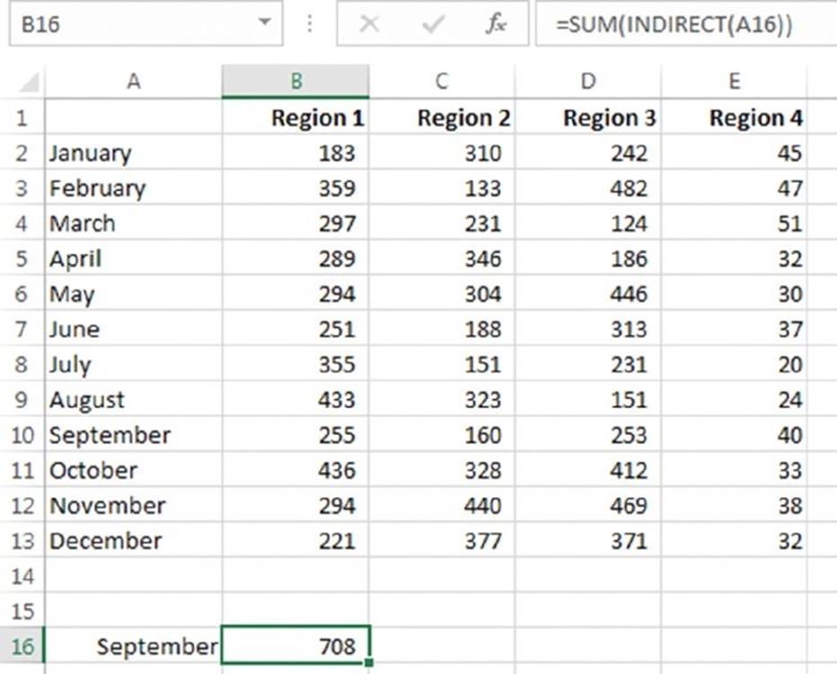
Figure 3.16 Using the INDIRECT function with a named range.

=SUM(INDIRECT(A16))

This formula returns the sum of the named range entered as text in cell A16.

Tip

You can use the Data ➜ Data Tools ➜ Data Validation command to insert a drop-down list box into cell A16. (Use the List option in the Data Validation dialog box and specify A2:A13 as the list source.) This allows the user to select a month name from a list; the total for the selected month then displays in B16.

On the Web

The workbook with this example is available at this book’s website. The filename is indirect functions.xlsx.

You can also reference worksheet-level names with the INDIRECT function. For example, suppose you have a number of worksheets named Region1, Region2, and so on. Each sheet contains a worksheet-level name called TotalSales. This formula retrieves the value from the appropriate sheet using the sheet name typed in cell A1:

=INDIRECT(A1&"!TotalSales")

If cell A1 contains the text Region2, the formula evaluates to the following:

=Region2!TotalSales

Using arrays in named formulas

An array is a collection of items. You can visualize an array as a single-column vertical collection, a single-row horizontal collection, or a multirow and multicolumn collection.

Cross-Ref

Part IV of this book, “Array Formulas,” discusses arrays and array formulas, but this topic is also relevant when discussing names.

You specify an array by using curly brackets. A comma or semicolon separates each item in the array. Use a comma to separate items arranged horizontally, and use a semicolon to separate items arranged vertically.

Use the New Name dialog box to create a formula named MonthNames that consists of the following formula definition:

={"Jan","Feb","Mar","Apr","May","Jun","Jul","Aug","Sep","Oct","Nov","Dec"}

This formula defines a 12-item array of text strings, arranged horizontally.

Note

When you type this formula, make sure that you include the brackets. Entering an array formula into the New Name dialog box is different from entering an array formula into a cell.

After you define the MonthNames formula, you can use it in a formula. However, your formula needs to specify which array item to use. The INDEX function is perfect for this. For example, the following formula returns Aug:

=INDEX(MonthNames,8)

You can also display the entire 12-item array, but it requires 12 adjacent cells to do so. For example, to enter the 12 items of the array into A3:L3, follow these steps (which assume that you used the New Name dialog box to create the formula named MonthNames):

1. Select the range A3:L3.

2. Type =MonthNames into the Formula bar.

3. Press Ctrl+Shift+Enter.

Pressing Ctrl+Shift+Enter tells Excel to insert an array formula into the selected cells. In this case, the single formula is entered into the selected adjacent cell. Excel places brackets around an array formula to remind you that it’s a special type of formula. If you examine any cell in A3:L3, you see its formula listed as follows:

{=MonthNames}

Notice that you can’t delete any of the months because the 12 cells make up a multicell array formula—a single formula that occupies multiple cells.

To insert the month names into A1:A12 (a vertical range), do the following:

1. Select the range A1:A12.

2. Type =TRANSPOSE(MonthNames) into the Formula bar.

3. Press Ctrl+Shift+Enter.

Creating a dynamic named formula

A dynamic named formula is a named formula that refers to a range not fixed in size. You may find this concept difficult to grasp, so a quick example is in order.

Examine the worksheet shown in Figure 3.17. This sheet contains a listing of sales by month, through the month of June.

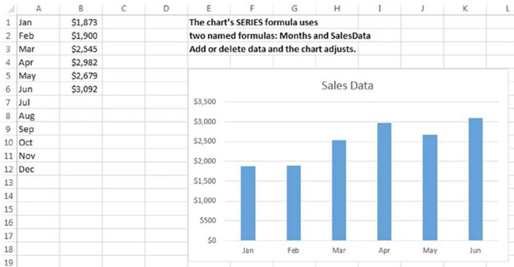
Figure 3.17 You can use a dynamic named formula to represent the sales data in column B.

Suppose you want to create a name (SalesData) for the data in column B, but you don’t want this name to refer to empty cells. In other words, the reference for the SalesData range would change each month as you add a new sales figure. You could, of course, use the Name Manager dialog box to change the range name definition each month. Or you could create a dynamic named formula that changes automatically as you enter new data.

To create a dynamic named formula, start by re-creating the worksheet shown in Figure 3.17. Then follow these steps:

1. Bring up the New Name dialog box.

2. Type SalesData into the Name field.

3. Type the following formula into the Refers To field:

=OFFSET(Sheet1!$B$1,0,0,COUNTA(Sheet1!$B:$B),1)

4. Click OK to close the New Name dialog box.

The preceding steps create a named formula that uses Excel’s OFFSET and COUNTA functions to return a range that changes, based on the number of nonempty cells in column B.

Note

This formula assumes that the range doesn’t contain blank cells. For example, if cell B2 is empty, the COUNTA function does not count that cell, and the OFFSET function returns an incorrect range.

To try out this formula, enter the following formula into any cell not in column B:

=SUM(SalesData)

This formula returns the sum of the values in column B. Note that SalesData does not display in the Name box and does not appear in the Go To dialog box. You can, however, type SalesData into the Name box to select the range. Or bring up the Go To dialog box and type SalesData to select the range.

At this point, you may be wondering about the value of this exercise. After all, a simple formula such as the following does the same job, without the need to define a formula:

=SUM(B:B)

Or you could just enter this formula directly into a cell without creating a named formula:

=SUM(OFFSET($B$1,0,0,COUNTA($B:$B),1))

The truth is, dynamic named formulas were more important in older versions of Excel. Dynamic named formulas used to be the only way to create a chart that adjusted automatically as you added new data. However, with the introduction of tables (created by using Insert ➜ Tables ➜ Table), dynamic named formulas are rarely necessary. If you create a chart from data in a table, the chart adjusts automatically.

Cross-Ref

Refer to Chapter 9, “Working with Tables and Lists,” for more information about tables.

On the Web

The workbook with this example is available at this book’s website. The filename is dynamic named formula.xlsx. The named formula is also used in a chart’s SERIES formula, creating a self-expanding chart.

Using an XLM macro in a named formula

The final example is both interesting—because it uses an Excel 4 XLM macro function in a named formula—and useful—because it’s a relatively simple way of getting a list of filenames into a worksheet.

Start with an empty workbook, and create a formula named FileList, defined as

=FILES(Sheet1!$A$1)

The FILES function is not a normal worksheet function. Rather, it’s an old XLM style macro function that is intended to be used on a special macro sheet. This function takes one argument (a directory path and file specification) and returns an array of filenames in that directory that match the file specification.

A normal worksheet formula cannot use these old XLM functions, but named formulas can.

After defining the named formula, enter a directory path and file specification into cell A1. For example:

E:\Backup\Excel\*.xl*

Then this formula displays the first file found:

=INDEX(FileList, 1)

If you change the second argument to 2, it displays the second file found, and so on.

Figure 3.18 shows an example. The path and filespec is in cell A1. Cell A2 contains this formula, copied down the column:

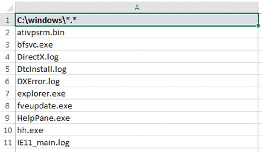
Figure 3.18 Using an XLM macro in a named formula can generate a list of file names in a worksheet.

=INDEX(FileList,ROW()-1)

The ROW function, as used here, generates a series of consecutive integers: 1, 2, 3, and so on. These integers are used as the second argument for the INDEX function. Note that cell A22 displays an error because the directory has only 20 files, and it’s attempting to display the twenty-first file.

When you change the directory or filespec in cell A1, the formulas update to display the new filenames.

On the Web

This workbook is available at this book’s website. The filename is file list.xlsm. You must enable macros when you open this workbook.