Excel 2016 Formulas (2016)
PART II
Leveraging Excel Functions
· Chapter 4: Introducing Worksheet Functions
· Chapter 5: Manipulating Text
· Chapter 6: Working with Dates and Times
· Chapter 7: Counting and Summing Techniques
· Chapter 8: Using Lookup Functions
· Chapter 9: Working with Tables and Lists
· Chapter 10: Miscellaneous Calculations
Chapter 4
Introducing Worksheet Functions
In This Chapter
· The advantages of using functions in your formulas
· The types of arguments used by functions
· How to enter a function into a formula
A thorough knowledge of Excel’s worksheet functions is essential for anyone who wants to master the art of formulas. This chapter provides an overview of the functions available for use in formulas.
What Is a Function?
A worksheet function is a built-in tool that you use in a formula. Worksheet functions allow you to perform calculations or operations that would otherwise be impossible. A typical function (such as SUM) takes one or more arguments and then returns a result. The SUM function, for example, accepts a range argument and then returns the sum of the values in that range.
You’ll find functions useful because they
§ Simplify your formulas
§ Permit formulas to perform otherwise impossible calculations
§ Speed up some editing tasks
§ Allow conditional execution of formulas—giving them rudimentary decision-making capability
The examples in the sections that follow demonstrate each of these points.
Simplify your formulas
Using a built-in function can simplify a formula significantly. For example, you might need to calculate the average of the values in 10 cells (A1:A10). Without the help of any functions, you would need to construct a formula like this:
=(A1+A2+A3+A4+A5+A6+A7+A8+A9+A10)/10
Not very pretty, is it? Even worse, you would need to edit this formula if you inserted a new row in the A1:A10 range and needed the new value to be included in the average. However, you can replace this formula with a much simpler one that uses the AVERAGE function:
=AVERAGE(A1:A10)
Perform otherwise impossible calculations
Functions permit formulas to perform calculations that go beyond the standard mathematical operations. Perhaps you need to determine the largest value in a range. A formula can’t tell you the answer without using a function. This formula uses the MAX function to return the largest value in the range A1:D100:
=MAX(A1:D100)
Speed up editing tasks
Functions can sometimes eliminate manual editing. Assume that you have a worksheet that contains 1,000 names in cells A1:A1000 and that all the names appear in all-uppercase letters. Your boss sees the listing and informs you that you need to mail-merge the names with a form letter and that the use of all uppercase is not acceptable. For example, JOHN F. CRANE must appear as John F. Crane. You could spend the rest of the afternoon reentering the list—or you could use a formula such as the following, which uses the PROPER function to convert the text in cell A1 to proper case:
=PROPER(A1)
1. Type this formula in cell B1 and then copy it down to the next 999 rows.
2. Select B1:B1000 and choose Home ➜ Clipboard ➜ Copy to copy the range to the Clipboard (or press Ctrl+C).
3. Activate cell A1 and choose Home ➜ Clipboard ➜ Paste ➜ Paste Values to convert the formulas to values.
4. Delete column B.
You’re finished! With the help of a function, you just eliminated several hours of tedious work in less than a minute.
![]() Note
Note
Excel 2013 introduced Flash Fill, which can sometimes take the place of formulas for text-conversion tasks like the one described here. See Chapter 16, “Importing and Cleaning Data,” for details.
Provide decision-making capability
You can use the Excel IF function to give your formulas decision-making capabilities. Suppose that you have a worksheet that calculates sales commissions. If a salesperson sells at least $100,000 of product, the commission rate reaches 7.5 percent; otherwise, the commission rate remains at 5.0 percent. Without using a function, you would need to create two different formulas and make sure that you use the correct formula for each sales amount. This formula uses the IF function to check the value in cell A1 and make the appropriate commission calculation:
=IF(A1<100000,A1*5%,A1*7.5%)
The IF function takes three arguments, each separated by a comma. These arguments provide input to the function. The formula is making a decision: if the value in cell A1 is less than 100,000, then return the value in cell A1 multiplied by 5 percent. Otherwise, return the value in cell A1 multiplied by 7.5 percent.
More about functions
All told, Excel 2016 includes more than 400 functions. And if that’s not enough, you can purchase additional specialized functions from third-party suppliers. You can even create your own custom functions using VBA.
![]() Cross-Ref
Cross-Ref
If you’re ready to create your own custom functions by using VBA, check out Part VI, “Developing Custom Worksheet Functions.”
The sheer number of available worksheet functions may overwhelm you, but you’ll probably find that you use only a dozen or so of the functions on a regular basis. And as you’ll see, the Function Library group on the Formulas tab (described later in this chapter) makes it easy to locate and insert a function, even if you use it only rarely.
![]() Cross-Ref
Cross-Ref
Appendix A, “Excel Function Reference,” contains a complete listing of Excel’s worksheet functions, with a brief description of each.
Function Argument Types
If you examine the preceding examples in this chapter, you’ll notice that all the functions use a set of parentheses. The information within the parentheses is the function’s arguments. Functions vary in the way they use arguments. A function may use
§ No arguments
§ A fixed number of arguments
§ An indeterminate number of arguments
§ Optional arguments
For example, the RAND function, which returns a random number between 0 and 1, doesn’t use an argument. Even if a function doesn’t require an argument, you must provide a set of empty parentheses when you use the function in a formula, like this:
=RAND()
If a function uses more than one argument, a comma separates the arguments. For example, the LARGE function, which returns the nth largest value in a range, uses two arguments. The first argument represents the range; the second argument represents the value for n. The formula that follows returns the third-largest value in the range A1:A100:
=LARGE(A1:A100,3)
![]() Note
Note
In some non-English versions of Excel, the character used to separate function arguments can be something other than a comma—for example, a semicolon. The examples in this book use a comma as the argument separator character.
The examples at the beginning of the chapter use cell or range references for arguments. Excel proves quite flexible when it comes to function arguments, however. The following sections demonstrate additional argument types for functions.
![]() Accommodating former Lotus 1-2-3 users
Accommodating former Lotus 1-2-3 users
If you've ever used any of the Lotus 1-2-3 spreadsheets (or any version of Corel's Quattro Pro), you may recall that these products require you to type an “at” sign (@) before a function name. Excel is smart enough to distinguish functions without your having to flag them with a symbol.
Because old habits die hard, however, Excel accepts @ symbols when you type functions in your formulas, but it removes them as soon as you enter the formula.
These other spreadsheet programs also use two dots (..) as a range reference operator—for example, A1. . A10. Excel allows you to use this notation when you type formulas, but it replaces the dots with its own range reference operator: a colon (:). In fact, you can use any number of dots as a range reference operator, even something like this: A1……… . . A10.
This accommodation goes only so far, however. Excel still insists that you use the standard Excel function names, and it doesn't recognize or translate the function names used in other spreadsheets. For example, if you enter the 1-2-3 @AVG function, Excel flags it as an error. (Excel's name for this function is AVERAGE.)
Names as arguments
As you’ve seen, functions can use cell or range references for their arguments. When Excel calculates the formula, it uses the current contents of the cell or range to perform its calculations. The SUM function returns the sum of its argument(s). To calculate the sum of the values in A1:A20, you can use this:
=SUM(A1:A20)
And, not surprisingly, if you’ve defined a name for A1:A20 (such as Sales), you can use the name in place of the reference:
=SUM(Sales)
![]() Cross-Ref
Cross-Ref
For more information about defining and using names, refer to Chapter 3, “Working with Names.”
Full-column or full-row as arguments
In some cases, you may find it useful to use an entire column or row as an argument. For example, the following formula sums all values in column B:
=SUM(B:B)
Using full-column and full-row references is particularly useful if the range that you’re summing changes—if you continually add new sales figures, for instance. If you do use an entire row or column, just make sure that the row or column doesn’t contain extraneous information that you don’t want to include in the sum.
And, make sure your formula isn’t in the column that’s being referenced. If the preceding SUM formula is in column B, it will generate a circular reference error.
You may think that using such a large range (a column consists of 1,048,576 cells) might slow down calculation time. Not true. Excel keeps track of the last-used row and last-used column and does not use cells beyond them when computing a formula result that references an entire column or row.
Literal values as arguments
A literal argument refers to a value or text string that you enter directly. For example, the SQRT function, which calculates the square root of a number, takes one argument. In the following example, the formula uses a literal value for the function’s argument:
=SQRT(225)
Using a literal argument with a simple function like this one usually defeats the purpose of using a formula. This formula always returns the same value, so you could just as easily replace it with the value 15. You may want to make an exception to this rule in the interest of clarity. For example, you may want to make it perfectly clear that the value in the cell is the square root of 225.
Using literal arguments makes more sense with formulas that use more than one argument. For example, the LEFT function (which takes two arguments) returns characters from the beginning of its first argument; the second argument specifies the number of characters. If cell A1 contains the text Budget, the following formula returns the first three letters (Bud):
=LEFT(A1,3)
Expressions as arguments
You can also use expressions as arguments. Think of an expression as a formula within a formula (but without the leading equal sign). When Excel encounters an expression as a function’s argument, it evaluates the expression and then uses the result as the argument’s value. Here’s an example:
=SQRT((A1^2)+(A2^2))
This formula uses the SQRT function, and its single argument consists of the following expression:
(A1^2)+(A2^2)
When Excel evaluates the formula, it first evaluates the expression in the argument and then computes the square root of the result. This expression squares the value in cell A1 and adds it to the square of the value in cell A2.
Other functions as arguments
Because Excel can evaluate expressions as arguments, it shouldn’t surprise you that these expressions can include other functions. Writing formulas that have functions within functions is sometimes known as nesting functions. Excel starts by evaluating the most deeply nested expression and works its way out.
Here’s an example of a nested function:
=SIN(RADIANS(B9))
The RADIANS function converts degrees to radians, the unit that all Excel trigonometric functions use. If cell B9 contains an angle in degrees, the RADIANS function converts it to radians, and then the SIN function computes the sine of the angle.
A formula can contain up to 64 levels of nested functions—a limit that will probably never be a factor.
Arrays as arguments
A function can also use an array as an argument. An array is a series of values separated by a comma and enclosed in curly brackets. The formula that follows uses the OR function with an array as an argument. The formula returns TRUE if cell A1 contains 1, 3, or 5.
=OR(A1={1,3,5})
![]() Cross-Ref
Cross-Ref
See Part IV, “Array Formulas,” for more information about working with arrays.
Often, using arrays can help simplify your formula. The following formula, for example, returns the same result as the previous formula but uses nested IF functions instead of an array:
=IF(A1=1,TRUE,IF(A1=3,TRUE,IF(A1=5,TRUE,FALSE)))
Ways to Enter a Function into a Formula
You can enter a function into a formula by typing it manually, by using the Function Library commands, or by using the Insert Function dialog box.
Entering a function manually
If you’re familiar with a particular function—that is, you know its correct spelling and the types of arguments that it takes—you may choose to simply type the function and its arguments into your formula. Often, this method is the most efficient.
However, you can also use the handy Formula AutoComplete feature. When you type an equal sign and the first letter of a function in a cell, Excel displays a drop-down list box of all the functions that begin with that letter and a ScreenTip with a brief description for the function (see Figure 4.1). You can continue typing the function to limit the list or use the arrow keys to select the function from the list. After you select the desired function, press Tab to insert the function and its opening parenthesis into the formula.
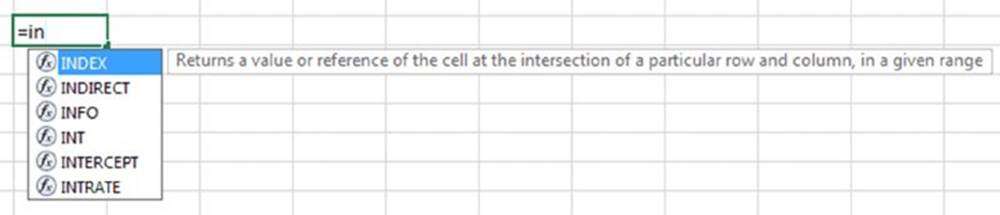
Figure 4.1 When you begin to type a function, Excel lists available functions that begin with the typed letters.
![]() Cross-Ref
Cross-Ref
In addition to displaying function names, the Formula AutoComplete feature lists cell and range names and table references. See Chapter 3 for information on names and Chapter 9, “Working with Tables and Lists,” for information about tables.
After you press Tab to insert the function and its opening parenthesis, Excel displays another ScreenTip that shows the arguments for the function (see Figure 4.2). The bold argument is the argument that you are entering. Arguments shown in square brackets are optional. Notice that the text in the ScreenTip contains a hyperlink for each argument that you’ve entered. Click a hyperlink to select the corresponding argument. If that ScreenTip gets in your way, you can drag it to a different location.
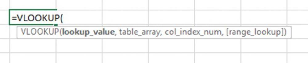
Figure 4.2 Excel displays a list of the function’s arguments.
If you don’t like using Formula AutoComplete, you can disable this feature. Choose File ➜ Options to display the Excel Options dialog box. On the Formulas tab, remove the check mark from the Formula AutoComplete option.
![]() Tip
Tip
When you type a built-in function, Excel always converts the function’s name to uppercase. Therefore, it’s a good idea to use lowercase when you type function names manually. If Excel doesn’t convert your text to uppercase after you press Enter, your entry isn’t recognized as a function, which means that you spelled it incorrectly or that the function isn’t available.
Using the Function Library commands
Another way to insert a function into a formula is to use the icons in the Formulas ➜ Function Library group. Figure 4.3 shows these icons, each of which is a drop-down control.
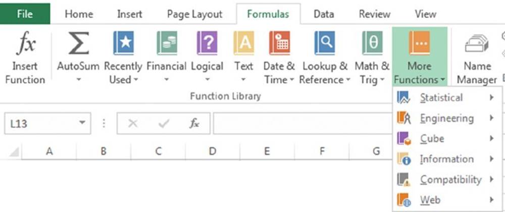
Figure 4.3 The icons in the Function Library group on the Formulas tab.
Each Function category is dedicated to a specific topic area.
· Financial functions: The financial functions enable you to perform common business calculations that deal with money. For example, you can use the PMT function to calculate the monthly payment for a car loan. You need to provide the loan amount, interest rate, and loan term as arguments.
· Date & Time functions: The functions in this category enable you to analyze and work with date and time values in formulas. For example, the TODAY function returns the current date (as stored in the system clock).
· Lookup & Reference functions: Functions in this category are used to find (look up) values in lists or tables. A common example is a tax table. For example, you can use the VLOOKUP function to determine a tax rate for a particular income level.
· Math & Trig functions: This category contains a variety of functions that perform mathematical and trigonometric calculations.
· Statistical functions: The functions in this category perform statistical analysis on ranges of data. For example, you can calculate statistics such as mean, mode, standard deviation, and variance.
· Text functions: Text functions enable you to manipulate text strings in formulas. For example, you can use the MID function to extract any number of characters beginning at any character position. Other functions enable you to change the case of text: convert to uppercase, for example.
· Logical functions: This category consists of only seven functions that enable you to test a condition, for logical TRUE or FALSE. You will find the IF function useful because it gives your formulas simple decision-making capabilities.
· Information functions: The functions in this category help you determine the type of data stored within a cell. For example, the ISTEXT function returns TRUE if a cell reference contains text. Or you can use the ISBLANK function to determine whether a cell is empty. The CELL function returns lots of potentially useful information about a particular cell.
· Engineering functions: The functions in this category can prove useful for engineering applications. They enable you to work with complex numbers and to perform conversions between various numbering and measurement systems.
· Cube functions: The functions in this category allow you to manipulate data that is part of an OLAP data cube.
· Compatibility functions: The Compatibility category was introduced in Excel 2010. Functions in this category are statistical functions that have been replaced with improved versions of themselves. These older functions are retained in Excel for the purpose of backward compatibility with Excel 2007 and prior versions.
· Web functions: The Web category was introduced in Excel 2013 and includes three functions that deal with Internet-related tasks like encoding URL addresses and parsing web services.
When you select a function from one of these lists, Excel displays its Function Arguments dialog box to help you enter the arguments. See the section, “Using the Insert Function dialog box” for more information about the Function Arguments dialog box.
![]()
In addition to the function categories described previously, Excel includes other categories that will not appear on the Excel Ribbon. These are Database functions, Commands, Customizing, Macro Control, and DDE/External. Although many of the functions found in these categories are holdovers from older versions of Excel, some of the functions still prove to be useful in some scenarios. For example, the Database functions come in handy when you need to summarize data in a table that meets specific criteria. See Chapter 9 for more information on Database functions.
Using the Insert Function dialog box
The Insert Function dialog box is another way to enter a function into a formula. Using the Insert Function dialog box ensures that you spell the function correctly and that it contains the proper number of arguments in the correct order.
To insert a function, select the function from the Insert Function dialog box, as shown in Figure 4.4. You access this dialog box in several ways:
§ Choose Formulas ➜ Function Library ➜ Insert Function.
§ Choose any icon category in the Formulas ➜ Function Library group, and select Insert Function from the drop-down list.
§ Click the fx icon to the left of the Formula bar.
§ Press Shift+F3.
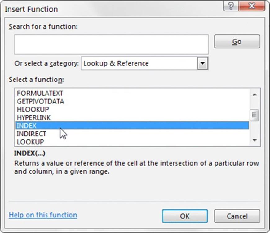
Figure 4.4 The Insert Function dialog box.
The Insert Function dialog box contains a drop-down list of categories. When you select a category from the list, the list box displays the functions in the selected category. The Most Recently Used category lists the functions that you’ve used most recently. The All category lists all the functions available across all categories. Access this category if you know a function’s name but not its category.
If you’re not sure which function to use, you can search for a function. Use the field at the top of the Insert Function dialog box. Type one or more keywords and click Go. Excel then displays a list of functions that match your search criteria. For example, if you’re looking for functions to calculate a loan payment, type loan as the search term.
When you select a function from the Select a Function list box, notice that Excel displays the function (and its argument names) in the dialog box, along with a brief description of what the function does. Also, you can click Help on This Function to read about the selected function in Excel’s Help system.
When you locate the function that you want to use, click OK. Excel’s Function Arguments dialog box appears, as shown in Figure 4.5, where you can specify the arguments for the function. To specify a cell or range as an argument, just click in the worksheet and point to the cell or range. Note that each argument is described.
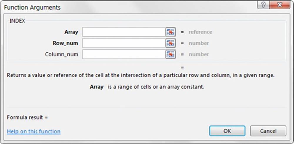
Figure 4.5 The Function Arguments dialog box.
When you choose Formulas ➜ Function Library ➜ AutoSum (or Home ➜ Editing ➜ AutoSum), Excel does a quick check of the surrounding cells. It then proposes a formula that uses the SUM function. If Excel guessed your intentions correctly, just press Enter to accept the proposed formula(s). If Excel guessed incorrectly, you can simply select the range with your mouse to override Excel’s suggestion (or press Esc to cancel the AutoSum).
You can preselect the cells to be included in an AutoSum rather than let Excel guess which cells you want. To insert a SUM function into cell A11 that sums A1:A10, select A1:A11 and then click the AutoSum button.
The AutoSum button displays an arrow that, when clicked, displays additional functions. For example, you can use this button to insert a formula that uses the AVERAGE function.
When you’re working with a table (created by using Insert ➜ Tables ➜ Table), you can choose Table Tools ➜ Design ➜ Total Row, and Excel displays a new row at the bottom of the table that contains summary formulas for the columns. See Chapter 9 for more information about tables.
When you choose Data ➜ Data Tools ➜ Outline ➜ Subtotal, Excel displays a dialog box that enables you to specify some options. Then it proceeds to insert rows and enter some formulas automatically. These formulas use the SUBTOTAL function.
More tips for entering functions
The following list contains some additional tips to keep in mind when you use the Insert Function dialog box to enter functions:
§ Click the Help on This Function link (lower left, Figure 4.5) to get help (see Figure 4.6) about the function that you selected.
§ If the active cell already contains a formula that uses a function, clicking the Insert Function button displays the Function Arguments dialog box.
§ You can use the Insert Function dialog box to insert a function into an existing formula. Just edit the formula and move the insertion point to the location where you want to insert the function. Then open the Insert Function dialog box and select the function.
§ If you change your mind about entering a function, click Cancel.
§ The number of arguments used by the function that you select determines the number of boxes that you see in the Function Arguments dialog box. If a function uses no arguments, you won’t see any boxes. If the function uses a variable number of arguments (as with the AVERAGE function), Excel adds a new box every time you enter an optional argument.
§ On the right side of each box in the Function Arguments dialog box, you’ll see the current value for each argument that’s entered or the type of argument (such as text or number) for arguments yet to be entered.
§ A few functions, such as INDEX, have more than one form. If you choose such a function, Excel displays the Select Arguments dialog box that enables you to choose which form you want to use.
§ To locate a function quickly in the Function Name list that appears in the Insert Function dialog box, open the list box, type the first letter of the function name, and then scroll to the desired function. For example, if you select the All category and want to insert the SIN function, click anywhere on the Select a Function list box and type S. Excel selects the first function that begins with S. Keep typing S (or press the down arrow key) until you reach the SIN function.
§ If the active cell contains a formula that uses one or more functions, the Function Arguments dialog box enables you to edit each function. In the Formula bar, click the function that you want to edit and then click the Insert Function button.
§ Some Excel functions are considered to be volatile. Volatile functions are those that recalculate whenever Excel recalculates the workbook, even if the formula that contains the function is not involved in the recalculation. It is by no means a bad thing to use functions that are volatile. Many of them are quite important to many data models. However, you should be aware of a minor side effect of using a volatile function: Excel will prompt you to save your workbook when you close it—even if you made no changes to it. For example, if you open a workbook that contains a volatile function, scroll around a bit (but don’t change anything) and then close the file, Excel will ask whether you want to save the workbook. The RAND function is an example of a volatile function. Think about how the RAND function generates a new random number every time Excel calculates the worksheet. Other examples of volatile functions include NOW, TODAY, OFFSET, INDIRECT, and CELL.
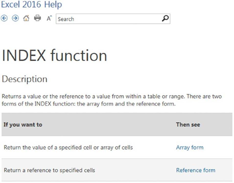
Figure 4.6 Don't forget about Excel's Help system. It's the most comprehensive function reference source available.
All materials on the site are licensed Creative Commons Attribution-Sharealike 3.0 Unported CC BY-SA 3.0 & GNU Free Documentation License (GFDL)
If you are the copyright holder of any material contained on our site and intend to remove it, please contact our site administrator for approval.
© 2016-2026 All site design rights belong to S.Y.A.