Excel 2016 Formulas (2016)
PART II
Leveraging Excel Functions
Chapter 8
Using Lookup Functions
In This Chapter
· An introduction to formulas that look up values in a table
· An overview of the worksheet functions used to perform lookups
· Basic lookup formulas
· More sophisticated lookup formulas
This chapter discusses various techniques that you can use to look up a value in a table. Microsoft Excel has three functions (LOOKUP, VLOOKUP, and HLOOKUP) designed for this task, but you may find that these functions don’t quite cut it. This chapter provides many lookup examples, including alternative techniques that go well beyond Excel’s normal lookup capabilities.
What Is a Lookup Formula?
A lookup formula essentially returns a value from a table (in a range) by looking up another related value. A common telephone directory (remember those?) provides a good analogy: if you want to find a person’s telephone number, you first locate the name (look it up) and then retrieve the corresponding number.
![]() Note
Note
Note that the term table is used here to describe a range of data. The range does not necessarily need to be an “official” table, as created by the Excel Insert ➜ Tables ➜Table command.
Figure 8.1 shows a simple worksheet that uses several lookup formulas. This worksheet contains a table of employee data (named EmpData). When you enter a last name into cell C2, lookup formulas in D2:G2 retrieve the matching information from the table. The lookup formulas in the following table use the VLOOKUP function.
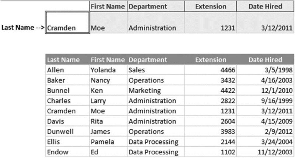
Figure 8.1 Lookup formulas in row 2 look up the information for the last name in cell C2.
|
Cell |
Formula |
|
D2 |
=VLOOKUP(C2,EmpData,2,FALSE) |
|
E2 |
=VLOOKUP(C2,EmpData,3,FALSE) |
|
F2 |
=VLOOKUP(C2,EmpData,4,FALSE) |
|
G2 |
=VLOOKUP(C2,EmpData,5,FALSE) |
This particular example uses four formulas to return information from the EmpData range. In many cases, you’ll want only a single value from the table, so use only one formula.
Functions Relevant to Lookups
Several Excel functions are useful when writing formulas to look up information in a table. Table 8.1 lists and describes each of these functions.
Table 8.1 Functions Used in Lookup Formulas
|
Function |
Description |
|
CHOOSE |
Returns a specific value from a list of values supplied as arguments. |
|
HLOOKUP |
Horizontal lookup. Searches for a value in the top row of a table and returns a value in the same column from a row you specify in the table. |
|
IF |
Returns one value if a condition you specify is TRUE, and returns another value if the condition is FALSE. |
|
IFERROR* |
If the first argument returns an error, the second argument is evaluated and returned. If the first argument does not return an error, then it is evaluated and returned. |
|
INDEX |
Returns a value (or the reference to a value) from within a table or range. |
|
LOOKUP |
Returns a value either from a one-row or one-column range. Another form of the LOOKUP function works like VLOOKUP (or HLOOKUP) but is restricted to returning a value from the last column (or row) of a range. |
|
MATCH |
Returns the relative position of an item in a range that matches a specified value. |
|
OFFSET |
Returns a reference to a range that is a specified number of rows and columns from a cell or range of cells. |
|
VLOOKUP |
Vertical lookup. Searches for a value in the first column of a table and returns a value in the same row from a column you specify in the table. |
* Introduced in Excel 2007.
The examples in this chapter use the functions listed in Table 8.1.
![]() Using the IF function for simple lookups
Using the IF function for simple lookups
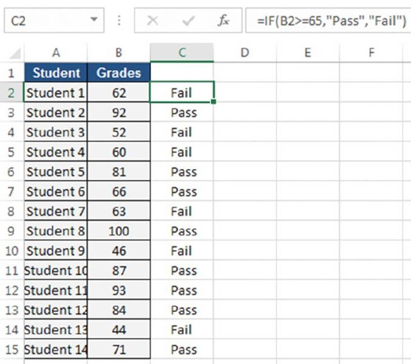
The IF function is versatile and is often suitable for simple decision-making problems. The accompanying figure shows a worksheet with student grades in column B. Formulas in column C use the IF function to return text: either Pass (a score of 65 or higher) or Fail (a score below 65). For example, the formula in cell C2 is
=IF(B2>=65,"Pass","Fail")
You can “nest” IF functions to provide even more decision-making ability. This formula, for example, returns one of four strings: Excellent, Very Good, Fair, or Poor:
=IF(B2>=90,"Excellent",IF(B2>=70,"Very Good",IF(B2>=50,"Fair","Poor")))
This technique is fine for situations that involve only a few choices. However, using nested IF functions can quickly become complicated and unwieldy. The lookup techniques described in this chapter usually provide a much better solution.
Basic Lookup Formulas
You can use Excel’s basic lookup functions to search a column or row for a lookup value to return another value as a result. Excel provides three basic lookup functions: HLOOKUP, VLOOKUP, and LOOKUP. The MATCH and INDEX functions are often used together to return a cell or relative cell reference for a lookup value.
![]() Note
Note
The examples in this section (plus the example in Figure 8.1) are available at this book’s website. The filename is basic lookup examples.xlsx.
The VLOOKUP function
The VLOOKUP function looks up the value in the first column of the lookup table and returns the corresponding value in a specified table column. The lookup table is arranged vertically. The syntax for the VLOOKUP function is
VLOOKUP(lookup_value,table_array,col_index_num,range_lookup)
The VLOOKUP function’s arguments are as follows:
§ lookup_value: The value that you want to look up in the first column of the lookup table.
§ table_array: The range that contains the lookup table.
§ col_index_num: The column number within the table from which the matching value is returned.
§ range_lookup: (Optional) If TRUE or omitted, an approximate match is returned. (If an exact match is not found, the next largest value that is less than lookup_value is used.) If FALSE, VLOOKUP searches for an exact match. If VLOOKUP cannot find an exact match, the function returns #N/A.
![]() Note
Note
If the range_lookup argument is TRUE or omitted, the first column of the lookup table must be in ascending order. If lookup_value is smaller than the smallest value in the first column of table_array, VLOOKUP returns #N/A. If the range_lookupargument is FALSE, the first column of the lookup table need not be in ascending order. If an exact match is not found, the function returns #N/A.
![]() Tip
Tip
If the lookup_value argument is text (and the fourth argument, range_lookup, is FALSE), you can include the wildcard characters * and ?. An asterisk matches any group of characters, and a question mark matches any single character.
The classic example of a lookup formula involves an income tax rate schedule (see Figure 8.2). The tax rate schedule shows the income tax rates for various income levels. The following formula (in cell B3) returns the tax rate for the income in cell B2:
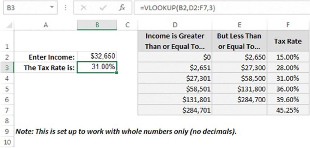
Figure 8.2 Using VLOOKUP to look up a tax rate.
=VLOOKUP(B2,D2:F7,3)
The lookup table resides in a range that consists of three columns (D2:F7). Because the third argument for the VLOOKUP function is 3, the formula returns the corresponding value in the third column of the lookup table.
Note that an exact match is not required. If an exact match is not found in the first column of the lookup table, the VLOOKUP function uses the next largest value that is less than the lookup value. In other words, the function uses the row in which the value you want to look up is greater than or equal to the row value but less than the value in the next row. In the case of a tax table, this is exactly what you want to happen.
The HLOOKUP function
The HLOOKUP function works just like the VLOOKUP function except that the lookup table is arranged horizontally instead of vertically. The HLOOKUP function looks up the value in the first row of the lookup table and returns the corresponding value in a specified table row.
The syntax for the HLOOKUP function is
HLOOKUP(lookup_value,table_array,row_index_num,range_lookup)
The HLOOKUP function’s arguments are as follows:
§ lookup_value: The value that you want to look up in the first row of the lookup table.
§ table_array: The range that contains the lookup table.
§ row_index_num: The row number within the table from which the matching value is returned.
§ range_lookup: (Optional) If TRUE or omitted, an approximate match is returned. (If an exact match is not found, the next largest value less than lookup_value is used.) If FALSE, VLOOKUP searches for an exact match. If VLOOKUP cannot find an exact match, the function returns #N/A.
![]() Tip
Tip
If the lookup_value argument is text (and the fourth argument is FALSE), you can use the wildcard characters * and ?. An asterisk matches any number of characters, and a question mark matches a single character.
Figure 8.3 shows the tax rate example with a horizontal lookup table (in the range E1:J3). The formula in cell B3 is
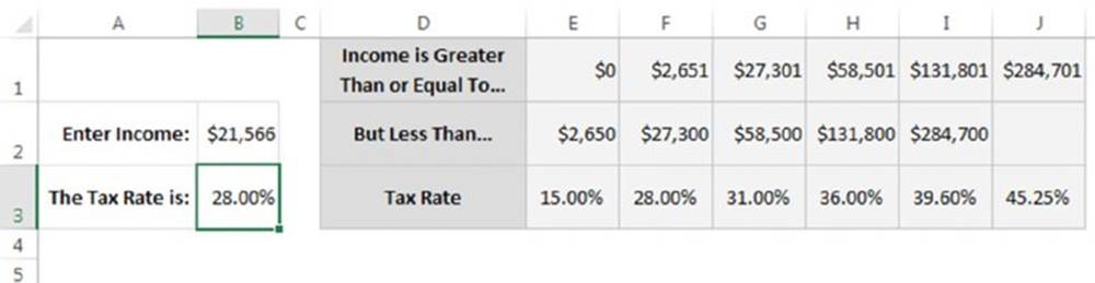
Figure 8.3 Using HLOOKUP to look up a tax rate.
=HLOOKUP(B2,E1:J3,3)
The LOOKUP function
The LOOKUP function has the following syntax:
LOOKUP(lookup_value,lookup_vector,result_vector)
The function’s arguments are as follows:
§ lookup_value: The value that you want to look up in the lookup_vector.
§ lookup_vector: A single-column or single-row range that contains the values to be looked up. These values must be in ascending order.
§ result_vector: The single-column or single-row range that contains the values to be returned. It must be the same size as the lookup_vector.
The LOOKUP function looks in a one-row or one-column range (lookup_vector) for a value (lookup_value) and returns a value from the same position in a second one-row or one-column range (result_vector).
![]() Warning
Warning
Values in the lookup_vector must be in ascending order. If lookup_value is smaller than the smallest value in lookup_vector, LOOKUP returns #N/A.
![]() Note
Note
The Help system also lists an “array” syntax for the LOOKUP function. This alternative syntax is included for compatibility with other spreadsheet products. In general, you can use the VLOOKUP or HLOOKUP functions rather than the array syntax.
Figure 8.4 shows the tax table again. This time, the formula in cell B3 uses the LOOKUP function to return the corresponding tax rate. The formula in B3 is
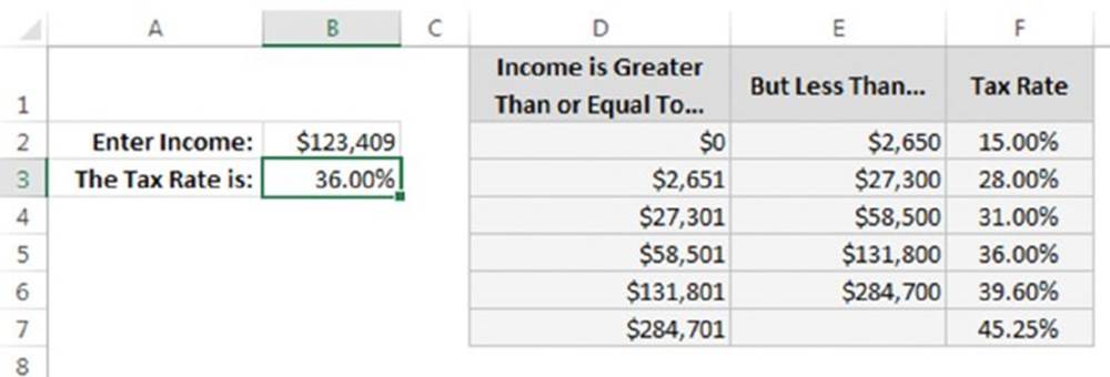
Figure 8.4 Using LOOKUP to look up a tax rate.
=LOOKUP(B2,D2:D7,F2:F7)
![]() Warning
Warning
If the values in the first column are not arranged in ascending order, the LOOKUP function may return an incorrect value.
Note that LOOKUP (as opposed to VLOOKUP) can return a value that’s in a different row than the matched value. If your lookup_vector and your result_vector are not part of the same table, LOOKUP can be a useful function. If, however, they are part of the same table, VLOOKUP is usually a better choice if for no other reason than that LOOKUP will not work on unsorted data.
Combining the MATCH and INDEX functions
The MATCH and INDEX functions are often used together to perform lookups. The MATCH function returns the relative position of a cell in a range that matches a specified value. The syntax for MATCH is
MATCH(lookup_value,lookup_array,match_type)
The MATCH function’s arguments are as follows:
§ lookup_value: The value that you want to match in lookup_array. If match_type is 0 and the lookup_value is text, this argument can include the wildcard characters * and ?.
§ lookup_array: The range that you want to search. This should be a one-column or one-row range.
§ match_type: An integer (–1, 0, or 1) that specifies how the match is determined.
![]() Note
Note
If match_type is 1, MATCH finds the largest value less than or equal to lookup_value (lookup_array must be in ascending order). If match_type is 0, MATCH finds the first value exactly equal to lookup_value. If match_type is –1, MATCH finds the smallest value greater than or equal to lookup_value (lookup_array must be in descending order). If you omit the match_type argument, this argument is assumed to be 1.
The INDEX function returns a cell from a range. The syntax for the INDEX function is
INDEX(array,row_num,column_num)
The INDEX function’s arguments are as follows:
§ array: A range
§ row_num: A row number within the array argument
§ column_num: A column number within the array argument
![]() Note
Note
If an array contains only one row or column, the corresponding row_num or column_num argument is optional.
Figure 8.5 shows a worksheet with dates, day names, and amounts in columns D, E, and F. When you enter a date in cell B1, the following formula (in cell B2) searches the dates in column D and returns the corresponding amount from column F. The formula in B2 is
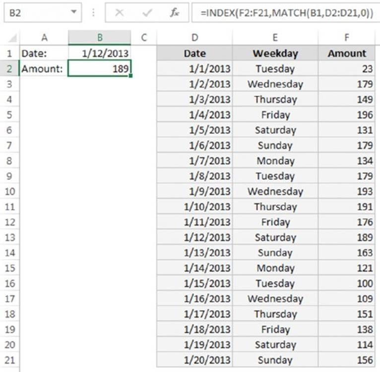
Figure 8.5 Using the INDEX and MATCH functions to perform a lookup.
=INDEX(F2:F21,MATCH(B1,D2:D21,0))
To understand how this formula works, start with the MATCH function. This function searches the range D2:D21 for the date in cell B1. It returns the relative row number where the date is found. This value is then used as the second argument for the INDEX function. The result is the corresponding value in F2:F21.
Specialized Lookup Formulas
You can use some additional types of lookup formulas to perform more specialized lookups. For instance, you can look up an exact value, search in another column besides the first in a lookup table, perform a case-sensitive lookup, return a value from among multiple lookup tables, and perform other specialized and complex lookups.
![]() On the Web
On the Web
The examples in this section are available at this book’s website. The filename is specialized lookup examples.xlsx.
Looking up an exact value
As demonstrated in the previous examples, VLOOKUP and HLOOKUP don’t necessarily require an exact match between the value to be looked up and the values in the lookup table. An example of an approximate match is looking up a tax rate in a tax table. In some cases, you may require a perfect match. For example, when looking up an employee number, you would probably require a perfect match for the number.
To look up an exact value only, use the VLOOKUP (or HLOOKUP) function with the optional fourth argument set to FALSE.
Figure 8.6 shows a worksheet with a lookup table that contains employee numbers (column A) and employee names (column B). The lookup table is named EmpList. The formula in cell B2, which follows, looks up the employee number entered into cell B1 and returns the corresponding employee name:

Figure 8.6 This lookup table requires an exact match.
=VLOOKUP(B1,EmpList,2,FALSE)
Because the last argument for the VLOOKUP function is FALSE, the function returns an employee name only if an exact match is found. If the employee number is not found, the formula returns #N/A. This, of course, is exactly what you want to happen because returning an approximate match for an employee number makes no sense. Also, notice that the employee numbers in column A are not in ascending order. If the last argument for VLOOKUP is FALSE, the values need not be in ascending order.
![]() Tip
Tip
If you prefer to see something other than #N/A when the employee number is not found, you can use the IFERROR function to test for the error result and substitute a different string. The following formula displays the text Not Found rather than#N/A:
=IFERROR(VLOOKUP(B1,EmpList,2,FALSE),"Not Found")
IFERROR works only with Excel 2007 and later. For compatibility with previous versions, use the following formula:
=IF(ISNA(VLOOKUP(B1,EmpList,2,FALSE)),"Not Found",
VLOOKUP(B1,EmpList,2,FALSE))
![]() When a blank is not a zero
When a blank is not a zero
Excel’s lookup functions treat empty cells in the result range as zeros. The worksheet in the accompanying figure contains a two-column lookup table, and the following formula looks up the name in cell B1 and returns the corresponding amount:
=VLOOKUP(E2,A2:B9,2,FALSE)
Note that the Amount cell for Charlie is blank, but the formula returns a 0.
If you need to distinguish zeros from blank cells, you must modify the lookup formula by adding an IF function to check whether the length of the returned value is 0. When the looked-up value is blank, the length of the return value is 0. In all other cases, the length of the returned value is nonzero. The following formula displays an empty string (a blank) whenever the length of the looked-up value is zero, and it displays the actual value whenever the length is anything but zero:
=IF(LEN(VLOOKUP(E2,A2:B9,2,FALSE))=0,"",(VLOOKUP(E2,A2:B9,2,FALSE)))
Alternatively, you can specifically check for an empty string, as in the following formula:
=IF(VLOOKUP(E2,A2:B9,2,FALSE)="","",(VLOOKUP(E2,A2:B9,2,FALSE)))
Looking up a value to the left
The VLOOKUP function always looks up a value in the first column of the lookup range. But what if you want to look up a value in a column other than the first column? It would be helpful if you could supply a negative value for the third argument for VLOOKUP—but you can’t.
Figure 8.7 illustrates the problem. Suppose you want to look up the batting average (column B, in a range named Average) of a player in column C (in a range named Player). The player you want data for appears in a cell named LookupValue. The VLOOKUP function won’t work because the data is not arranged correctly. One option is to rearrange your data, but sometimes that’s not possible.
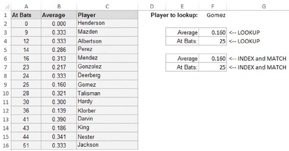
Figure 8.7 The VLOOKUP function can’t look up a value in column B based on a value in column C.
Another solution is to use the LOOKUP function, which requires two range arguments. The following formula (in cell F3) returns the batting average from column B of the player name contained in the cell named LookupValue:
=LOOKUP(LookupValue,Players,Averages)
Using the LOOKUP function requires the lookup range (in this case, the Players range) to be in ascending order. In addition to this limitation, the formula suffers from a slight problem: if you enter a nonexistentplayer—in other words, the LookupValue cell contains a value not found in the Players range—the formula returns an erroneous result.
A better solution uses the INDEX and MATCH functions. The formula that follows works just like the previous one except that it returns #N/A if the player is not found. Another advantage to using this formula is that the player names don’t need to be sorted:
=INDEX(Averages,MATCH(LookupValue,Players,0))
Performing a case-sensitive lookup
Excel’s lookup functions (LOOKUP, VLOOKUP, and HLOOKUP) are not case sensitive. For example, if you write a lookup formula to look up the text budget, the formula considers any of the following a match: BUDGET, Budget, or BuDgEt.
Figure 8.8 shows a simple example. Range D2:D9 is named Range1, and range E2:E9 is named Range2. The word to be looked up appears in cell B1 (named Value).
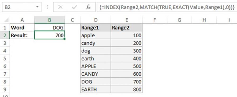
Figure 8.8 Using an array formula to perform a case-sensitive lookup.
The array formula that follows is in cell B2. This formula does a case-sensitive lookup in Range1 and returns the corresponding value in Range2.
{=INDEX(Range2,MATCH(TRUE,EXACT(Value,Range1),0))}
The formula looks up the word DOG (uppercase) and returns 700. The following standard LOOKUP formula (which is not case sensitive) returns 300:
=LOOKUP(Value,Range1,Range2)
![]() Note
Note
When entering an array formula, remember to use Ctrl+Shift+Enter, and do not type the curly brackets.
Choosing among multiple lookup tables
You can, of course, have any number of lookup tables in a worksheet. In some cases, your formula may need to decide which lookup table to use. Figure 8.9 shows an example.
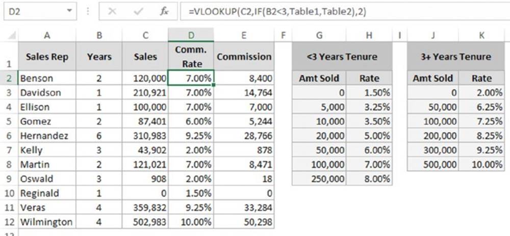
Figure 8.9 This worksheet demonstrates the use of multiple lookup tables.
This workbook calculates sales commission and contains two lookup tables: G3:H9 (named Table1) and J3:K8 (named Table2). The commission rate for a particular sales representative depends on two factors: the sales rep’s years of service (column B) and the amount sold (column C). Column D contains formulas that look up the commission rate from the appropriate table. For example, the formula in cell D2 is
=VLOOKUP(C2,IF(B2<3, Table1, Table2),2)
The second argument for the VLOOKUP function consists of an IF function that uses the value in column B to determine which lookup table to use.
The formula in column E simply multiplies the sales amount in column C by the commission rate in column D. The formula in cell E2, for example, is
=C2*D2
Determining letter grades for test scores
A common use of a lookup table is to assign letter grades for test scores. Figure 8.10 shows a worksheet with student test scores. The range E2:F6 (named GradeList) displays a lookup table used to assign a letter grade to a test score.
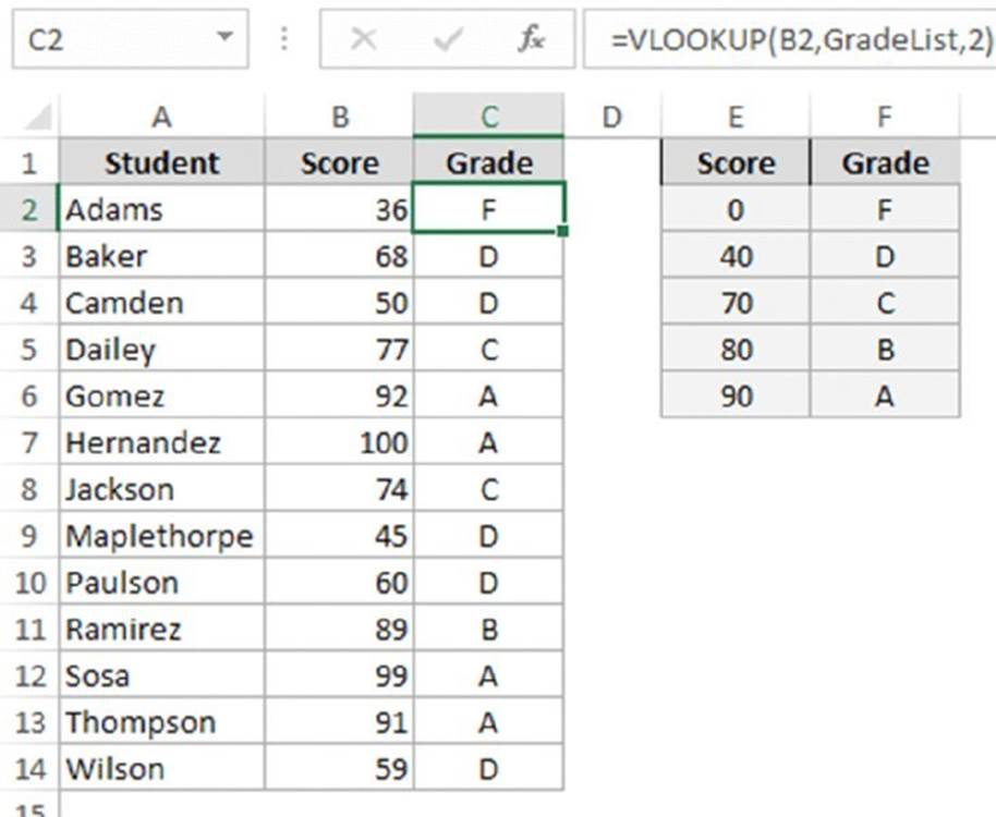
Figure 8.10 Looking up letter grades for test scores.
Column C contains formulas that use the VLOOKUP function and the lookup table to assign a grade based on the score in column B. The formula in C2, for example, is
=VLOOKUP(B2,GradeList,2)
When the lookup table is small (as in the example shown in Figure 8.10), you can use a literal array in place of the lookup table. The formula that follows, for example, returns a letter grade without using a lookup table. Instead, the information in the lookup table is hard-coded into an array constant. See Chapter 14, “Introducing Arrays,” for more information about array constants:
=VLOOKUP(B2,{0,"F";40,"D";70,"C";80,"B";90,"A"},2)
Another approach, which uses a more legible formula, is to use the LOOKUP function with two array arguments:
=LOOKUP(B2,{0,40,70,80,90},{"F","D","C","B","A"})
Calculating a grade point average
A student’s grade point average (GPA) is a numerical measure of the average grade received for classes taken. This discussion assumes a letter grade system, in which each letter grade is assigned a numeric value (A=4, B=3, C=2, D=1, and F=0). The GPA comprises an average of the numeric grade values, weighted by the credit hours of the course. A one-hour course, for example, receives less weight than a three-hour course. The GPA ranges from 0 (all Fs) to 4.00 (all As).
Figure 8.11 shows a worksheet with information for a student. This student took five courses, for a total of 13 credit hours. Range B2:B6 is named Credit Hrs. The grades for each course appear in column C (Range C2:C6 is named Grade). Column D uses a lookup formula to calculate the grade value for each course. The lookup formula in cell D2, for example, follows. This formula uses the lookup table in G2:H6 (named GradeTable).
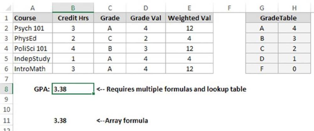
Figure 8.11 Using multiple formulas to calculate a GPA.
=VLOOKUP(C2,GradeTable,2,FALSE)
Formulas in column E calculate the weighted values. The formula in E2 is
=D2*B2
Cell B8 computes the GPA by using the following formula:
=SUM(E2:E6)/SUM(B2:B6)
The preceding formulas work fine, but you can streamline the GPA calculation quite a bit. In fact, you can use a single array formula to make this calculation and avoid using the lookup table and the formulas in columns D and E. This array formula does the job:
{=SUM((MATCH(Grades,{"F","D","C","B","A"},0)-1)*CreditHours)/SUM(CreditHours)}
Performing a two-way lookup
Figure 8.12 shows a worksheet with a table that displays product sales by month. To retrieve sales for a particular month and product, the user enters a month in cell B1 and a product name in cell B2.
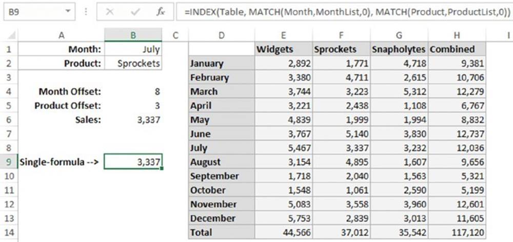
Figure 8.12 This table demonstrates a two-way lookup.
To simplify things, the worksheet uses the following named ranges:
|
Name |
Refers To |
|
Month |
B1 |
|
Product |
B2 |
|
Table |
D1:H14 |
|
MonthList |
D1:D14 |
|
ProductList |
D1:H1 |
The following formula (in cell B4) uses the MATCH function to return the position of the month within the MonthList range. For example, if the month is January, the formula returns 2 because January is the second item in the MonthList range. (The first item is a blank cell, D1.)
=MATCH(Month,MonthList,0)
The formula in cell B5 works similarly but uses the ProductList range:
=MATCH(Product,ProductList,0)
The final formula, in cell B6, returns the corresponding sales amount. It uses the INDEX function with the results from cells B4 and B5:
=INDEX(Table,B4,B5)
You can combine these formulas into a single formula, as shown here:
=INDEX(Table,MATCH(Month,MonthList,0),MATCH(Product,ProductList,0))
![]() Tip
Tip
Another way to accomplish a two-way lookup is to provide a name for each row and column of the table. A quick way to do this is to select the table and choose Formulas➜ Defined Names ➜ Create from Selection. After creating the names, you can use a simple formula to perform the two-way lookup, such as this:
=Sprockets July
This formula, which uses the range intersection operator (a space), returns July sales for Sprockets.
See Chapter 3, “Working with Names,” for details about the range intersection operator.
Performing a two-column lookup
Some situations may require a lookup based on the values in two columns. Figure 8.13 shows an example.
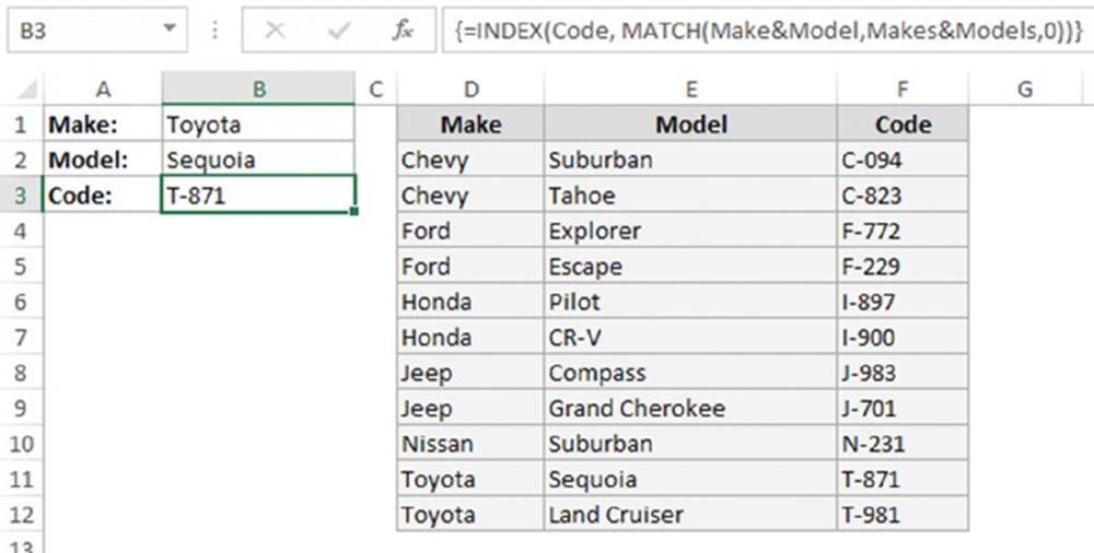
Figure 8.13 This workbook performs a lookup by using information in two columns (D and E).
The lookup table contains automobile makes and models and a corresponding code for each. The worksheet uses named ranges, as shown here:
|
F2:F12 |
Code |
|
B1 |
Make |
|
B2 |
Model |
|
D2:D12 |
Makes |
|
E2:E12 |
Models |
The following array formula displays the corresponding code for an automobile make and model:
{=INDEX(Code,MATCH(Make&Model,Makes&Models,0))}
This formula works by concatenating the contents of Make and Model and then searching for this text in an array consisting of the concatenated corresponding text in Makes and Models.
Determining the address of a value within a range
Most of the time, you want your lookup formula to return a value. You may, however, need to determine the cell address of a particular value within a range. For example, Figure 8.14 shows a worksheet with a range of numbers that occupy a single column (namedData). Cell B1, which contains the value to look up, is named Target.
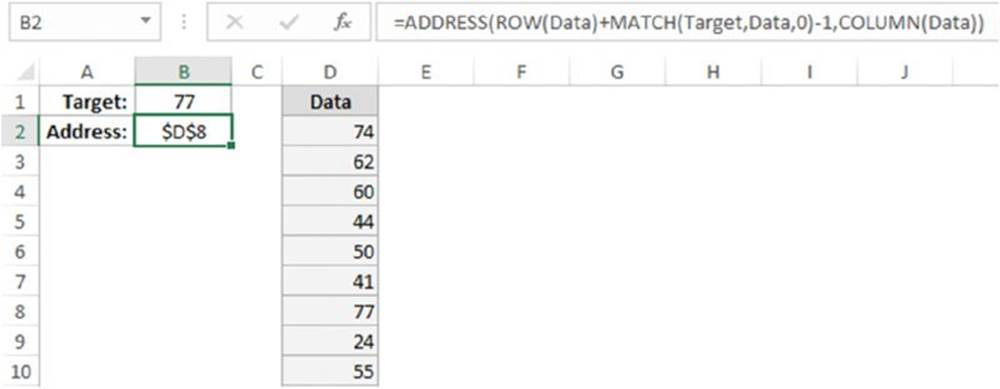
Figure 8.14 The formula in cell B2 returns the address in the Data range for the value in cell B1.
The formula in cell B2, which follows, returns the address of the cell in the Data range that contains the Target value:
=ADDRESS(ROW(Data)+MATCH(Target,Data,0)-1,COLUMN(Data))
If the Data range occupies a single row, use this formula to return the address of the Target value:
=ADDRESS(ROW(Data),COLUMN(Data)+MATCH(Target,Data,0)-1)
If the Data range contains more than one instance of the Target value, the address of the first occurrence is returned. If the Target value is not found in the Data range, the formula returns #N/A.
Looking up a value by using the closest match
The VLOOKUP and HLOOKUP functions are useful in the following situations:
§ You need to identify an exact match for a target value. Use FALSE as the function’s fourth argument.
§ You need to locate an approximate match. If the function’s fourth argument is TRUE or omitted, and an exact match is not found, the next largest value that is less than the lookup value is used.
But what if you need to look up a value based on the closest match? Neither VLOOKUP nor HLOOKUP can do the job.
Figure 8.15 shows a worksheet with student names in column A and data values in column B. Range B2:B20 is named Data. Cell E2, named Target Value, contains a value to search for in the Data range. Cell E3, named Column Offset, contains a value that represents the column offset from the Data range.
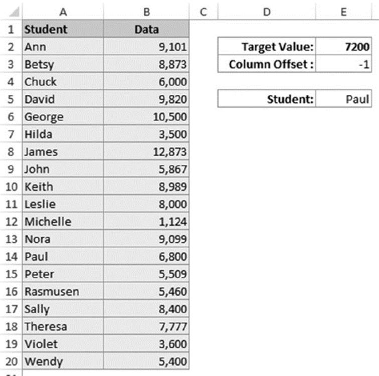
Figure 8.15 This workbook demonstrates how to perform a lookup by using the closest match.
The array formula that follows identifies the closest match to the Target Value in the Data range and returns the names of the corresponding student in column A (that is, the column with an offset of –1). The formula returns Paul (with a corresponding value of 6,800, which is the one closest to the Target Value of 7,200).
{=INDIRECT(ADDRESS(ROW(Data)+MATCH(MIN(ABS(Target-Data)),
ABS(Target-Data),0)-1,COLUMN(Data)+ColOffset))}
If two values in the Data range are equidistant from the Target Value, the formula uses the first one in the list.
The value in Column Offset can be negative (for a column to the left of Data), positive (for a column to the right of Data), or 0 (for the actual closest match value in the Data range).
To understand how this formula works, you need to understand the INDIRECT function. This function’s first argument is a text string in the form of a cell reference (or a reference to a cell that contains a text string). In this example, the text string is created by the ADDRESS function, which accepts a row and column reference and returns a cell address.
Looking up a value using linear interpolation
Interpolation refers to the process of estimating a missing value by using existing values. For an illustration of this concept, see Figure 8.16. Column D contains a list of values (named x), and column E contains corresponding values (named y).
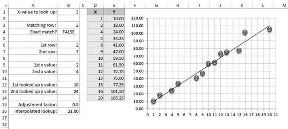
Figure 8.16 This worksheet demonstrates a table lookup using linear interpolation.
The worksheet also contains a chart that depicts the relationship between the x range and the y range graphically, and it includes a linear trendline. As you can see, an approximate linear relationship exists between the corresponding values in the x and y ranges: as xincreases, so does y. Notice that the values in the x range are not strictly consecutive. For example, the x range doesn’t contain the following values: 3, 6, 7, 14, 17, 18, and 19.
You can create a lookup formula that looks up a value in the x range and returns the corresponding value from the y range. But what if you want to estimate the y value for a missing x value? A normal lookup formula does not return a very good result because it simply returns an existing y value (not an estimated y value). For example, the following formula looks up the value 3 and returns 18.00 (the value that corresponds to 2 in the x range):
=LOOKUP(3,x,y)
In such a case, you probably want to interpolate. In other words, because the lookup value (3) is halfway between existing x values (2 and 4), you want the formula to return a y value of 21.00—a value halfway between the corresponding y values 18.00 and 24.00.
Formulas to perform a linear interpolation
Figure 8.17 shows a worksheet with formulas in column B. The value to be looked up is entered into cell B1. The final formula, in cell B16, returns the result. If the value in B3 is found in the x range, the corresponding y value is returned. If the value in B3 is not found, the formula in B16 returns an estimated y value, obtained using linear interpolation.
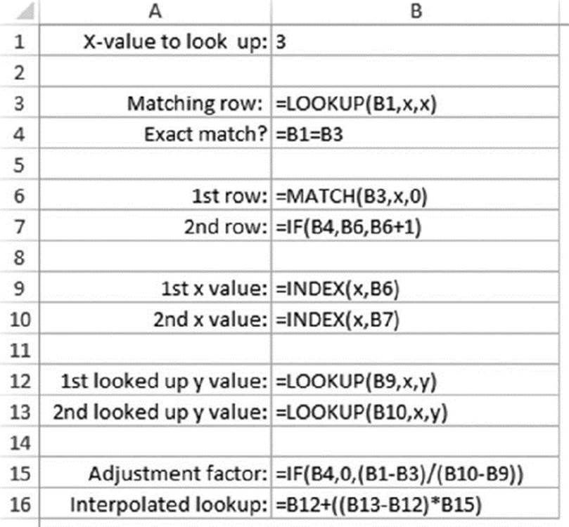
Figure 8.17 Column B contains formulas that perform a lookup using linear interpolation.
It’s critical that the values in the x range appear in ascending order. If B1 contains a value less than the lowest value in x or greater than the largest value in x, the formula returns an error value. Table 8.2 lists and describes these formulas.
Table 8.2 Formulas for a Lookup Using Linear Interpolation
|
Cell |
Formula |
Description |
|
B3 |
=LOOKUP(B1,x,x) |
Performs a standard lookup on the x range and returns the looked-up value. |
|
B4 |
=B1=B3 |
Returns TRUE if the looked-up value equals the value to be looked up. |
|
B6 |
=MATCH(B3,x,0) |
Returns the row number of the x range that contains the matching value. |
|
B7 |
=IF(B4,B6,B6+1) |
Returns the same row as the formula in B6 if an exact match is found. Otherwise, it adds 1 to the result in B6. |
|
B9 |
=INDEX(x,B6) |
Returns the x value that corresponds to the row in B6. |
|
B10 |
=INDEX(x,B7) |
Returns the x value that corresponds to the row in B7. |
|
B12 |
=LOOKUP(B9,x,y) |
Returns the y value that corresponds to the x value in B9. |
|
B13 |
=LOOKUP(B10,x,y) |
Returns the y value that corresponds to the x value in B10. |
|
B15 |
=IF(B4,0,(B1-B3)/(B10-B9)) |
Calculates an adjustment factor based on the difference between the x values. |
|
B16 |
=B12+((B13-B12)*B15) |
Calculates the estimated y value using the adjustment factor in B15. |
Combining the lookup and trend functions
Another slightly different approach, which you may find preferable to performing lookup using linear interpolation, uses the LOOKUP and TREND functions. One advantage is that it requires only one formula (see Figure 8.18).
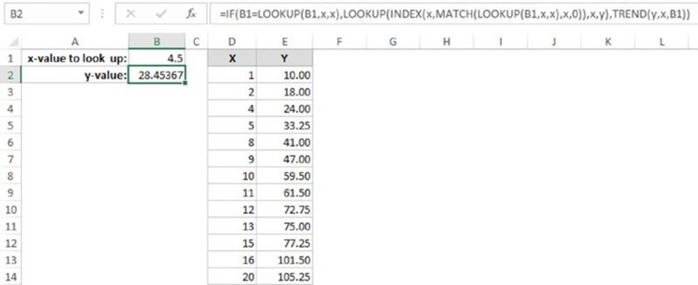
Figure 8.18 This worksheet uses a formula that uses the LOOKUP function and the TREND function.
The formula in cell B2 follows. This formula uses an IF function to make a decision. If an exact match is found in the x range, the formula returns the corresponding y value (using the LOOKUP function). If an exact match is not found, the formula uses the TREND function to return the calculated “best-fit” y value. (It does not perform a linear interpolation.)
=IF(B1=LOOKUP(B1,x,x),LOOKUP(INDEX(x,MATCH(LOOKUP(B1,x,x),x,0)),x,y),TREND(y,x,B1))
All materials on the site are licensed Creative Commons Attribution-Sharealike 3.0 Unported CC BY-SA 3.0 & GNU Free Documentation License (GFDL)
If you are the copyright holder of any material contained on our site and intend to remove it, please contact our site administrator for approval.
© 2016-2026 All site design rights belong to S.Y.A.