Excel 2016 Formulas (2016)

PART II
Leveraging Excel Functions

Chapter 9
Working with Tables and Lists

In This Chapter

· Using Excel’s table feature

· Basic information about using tables and lists

· Filtering data using simple criteria

· Using advanced filtering to filter data by specifying more complex criteria

· Understanding how to create a criteria range for use with advanced filtering or database functions

· Using the SUBTOTAL function to summarize data in a table

A list is a rectangular range of data that usually has a row of text headings to describe the contents of each column. Excel 2007 introduced a twist by letting you designate such a range as an “official” table, which makes common tasks much easier. More importantly, this table feature may eliminate some errors.

This chapter discusses Excel tables and covers what we refer to as lists, which are essentially tables of data that have not been converted to an official table.

Tables and Terminology

It seems that Microsoft can’t quite make up its mind when it comes to naming some of Excel’s features. Excel 2003 introduced a feature called lists, which is a way of working with what is sometimes called a worksheet database. In Excel 2007, the list features evolved into a much more useful feature called tables, and that feature was enhanced a bit in Excel 2010. To confuse the issue even more, Excel also has a feature called data tables, which has nothing at all to do with the table feature. And don’t forget about pivot tables, which are not actual tables but can be created from a table.

In this chapter, we use these two terms:

§ List: An organized collection of information contained in a rectangular range of cells. More specifically, a list comprises a row of headers (descriptive text), followed by additional rows of data holding values or text.

§ Table: A list that has been converted to a special type of range by using the Insert ➜ Tables ➜ Table command. Converting a list into an official table offers several advantages (and a few disadvantages), as we explain in this chapter.

A list example

Figure 9.1 shows a small list that contains employee information. It consists of a Header row, seven columns, and several rows of data. Notice that the data consists of different data types: text, numerical values, dates, and logical values. Column E even contains a formula that calculates the monthly salary from the value in column D.

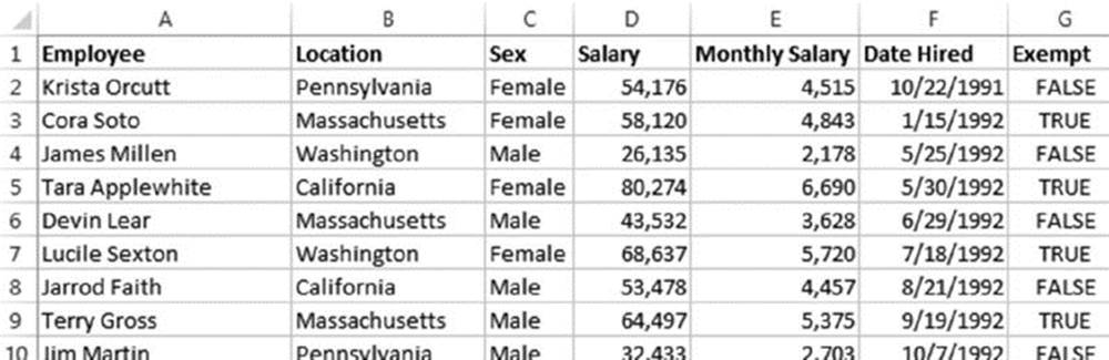
Figure 9.1 A typical list.

You can do lots of things with this list. You can sort it, filter it, create a chart from it, create subtotals, summarize it with a pivot table, and even remove duplicate rows (if it had any duplicate rows). A list like this is a common way to handle structured data.

A table example

Figure 9.2 shows the employee list after we converted it to a table, using Insert ➜ Tables ➜ Table. The table looks similar to a list, and the most obvious difference is the formatting (which was applied automatically).

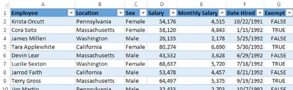
Figure 9.2 A list, converted to a table.

Apart from cosmetics, what’s the difference between a list and a table?

§ Activating any cell in the table gives you access to the Table Tools contextual tab on the Ribbon.

§ You can easily add a summary row at the bottom that summarizes the columns. When a summary row is present, Excel creates summary formulas automatically.

§ The table is assigned a name automatically (for example, Table1), and the range name adjusts automatically when you add or remove rows. You can change the name of the table using Formulas ➜ Defined Names ➜ Name Manager, but you cannot delete the name or change its definition. Note that the range name definition does not include the Header row or Total row.

§ The cells contain background color and text color formatting, applied automatically by Excel. This formatting is optional. The formatting is done by named table styles, which are customizable and tied to the workbook theme.

§ Each column header contains a Filter button that, when clicked, displays a drop-down list with sorting and filtering options. You can get this same functionality in a list by choosing Data ➜ Sort & Filter ➜ Filter.

§ You can add “Slicers” to make it easy for novices to filter the table. This feature was added with the release of Excel 2013.

§ If you scroll the worksheet down so that the Header row disappears, the table headers replace the column letters in the worksheet header. In other words, you don’t need to “freeze” the top row to keep the column labels visible when you scroll down.

§ Tables support calculated columns. A single formula entered into a column is propagated automatically to all cells in the column.

§ If you create a chart from data in a table, the chart series expands automatically after you add new data.

§ Tables support structured references. Rather than using cell references, formulas can use table names and column headers.

§ When you move your mouse pointer to the lower-right corner of the lower-right cell, you can click and drag to extend the table’s size horizontally (add more columns) or vertically (add more rows).

§ Excel is able to remove duplicate rows automatically. You can get this same functionality in a list by choosing Data ➜ Data Tools ➜ Remove Duplicates.

§ If your company uses Microsoft’s SharePoint service, you can easily publish a table to your SharePoint server. Choose Table Tools Design ➜ External Table Data ➜Export ➜ Export Table to SharePoint List.

§ Selecting rows and columns within the table is simplified.

Table limitations

Although an Excel table offers several advantages over a normal list, the Excel designers did impose some restrictions and limitations on tables. These limitations include the following:

· If a workbook contains a table, you cannot create or use custom views in that workbook (View ➜ Workbook Views ➜ Custom Views).

· A table cannot contain multicell array formulas.

· You cannot insert automatic subtotals (Data ➜ Outline ➜ Subtotal).

· You cannot share a workbook that contains a table (Review ➜ Changes ➜ Protect and Share Workbook).

· You cannot track changes in a workbook that contains a table (Review ➜ Changes ➜ Track Changes).

· You cannot use the Home ➜ Alignment ➜ Merge & Center command cells in a table (which makes sense because doing so would break up the rows or columns).

· You cannot use Flash Fill within a table.

If you encounter any of these limitations, just convert the table back to a list by using Table Tools ➜ Design ➜ Tools ➜ Convert to Range.

Working with Tables

It may take you a while to get used to working with tables, but you’ll soon discover that a table offers many advantages over a standard list.

The sections that follow cover common operations that you perform with a table.

Creating a table

Although Excel allows you to create a table from an empty range, most of the time you’ll create a table from an existing range of data (a list). The following instructions assume that you already have a range of data suitable for a table.

1. Make sure that the range doesn’t contain any completely blank rows or columns.

2. Activate any cell within the range.

3. Choose Insert ➜ Tables ➜ Table (or press Ctrl+T).

Excel responds with its Create Table dialog box. Excel tries to guess the range and whether the table has a Header row. Most of the time, it guesses correctly. If not, make your corrections before you click OK.

4. Click OK.

The table is automatically formatted, and Filter mode for the table is enabled. In addition, Excel displays its Table Tools contextual tab (as shown in Figure 9.3). The controls on this tab are relevant to working with a table.

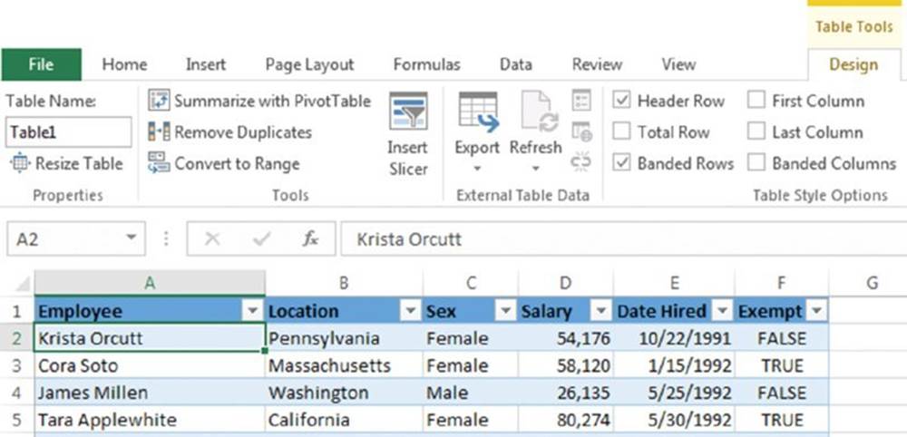
Figure 9.3 When you select a cell in a table, you can use the commands on the Table Tools contextual tab.

Tip

Another method for converting a range into a table is Home ➜ Styles ➜ Format as Table. This command name is a bit misleading. Choosing this command not only formats a range as a table but makes the range a table.

In the Create Table dialog box, Excel may guess the table’s dimensions incorrectly if the table isn’t separated from other information by at least one empty row or column. If Excel guesses incorrectly, just specify the exact range for the table in the dialog box. Or, click Cancel and rearrange your worksheet such that the table is separated from your other data by at least one blank row or column.

To create a table from an empty range, just select the range and choose Insert ➜ Tables ➜ Table. Excel creates the table, adds generic column headers (such as Column1 and Column2), and applies table formatting to the range. Almost always, you’ll want to replace the generic column headers with more meaningful text.

Changing the look of a table

When you create a table, Excel applies the default table style. The actual appearance depends on which document theme you use in the workbook. If you prefer a different look, you can easily change the entire look of the table.

Select any cell in the table and choose Table Tools ➜ Design ➜ Table Styles. The Ribbon shows one row of styles, but if you click the bottom of the vertical scrollbar, the Table Styles group expands, as shown in Figure 9.4. The styles are grouped into three categories: Light, Medium, and Dark. Notice that you get a live preview as you move your mouse among the styles. When you see one that you like, just click to make it permanent.

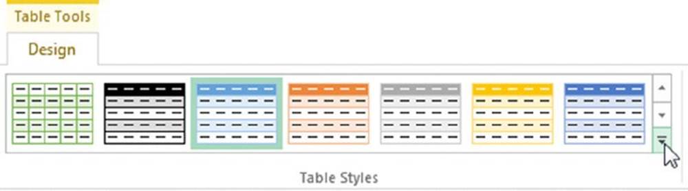
Figure 9.4 Excel offers many different table styles.

For a different set of color choices, choose Page Layout ➜ Themes ➜ Themes to select a different document theme.

Tip

If applying table styles isn’t working, the range was probably already formatted before you converted it to a table. (Table formatting doesn’t override normal formatting.) To clear the existing background fill colors, select the entire table and choose Home ➜ Font ➜ Fill Color ➜ No Fill. To clear the existing font colors, choose Home ➜ Font ➜Font Color ➜ Automatic. After you issue these commands, the table styles should work as expected.

You can change some elements of the style by using the check box controls of the Table Tools ➜ Design ➜ Table Style Options group. These controls determine whether various elements of the table are displayed and whether some formatting options are in effect:

§ Header Row: Toggles the display of the Header Row.

§ Total Row: Toggles the display of the Total Row.

§ First Column: Toggles special formatting for the first column. Depending on the table style used, this command might have no effect.

§ Last Column: Toggles special formatting for the last column. Depending on the table style used, this command might have no effect.

§ Banded Rows: Toggles the display of banded (alternating color) rows.

§ Banded Columns: Toggles the display of banded columns.

§ Filter Button: Toggles the display of the drop-down buttons in the table’s Header row.

Navigating and selecting in a table

Moving among cells in a table works just like moving among cells in a normal range. One difference is when you use the Tab key. When the active cell is in a table, pressing Tab moves to the cell to the right, as it normally does. But when you reach the last column, pressing Tab again moves to the first cell in the next row.

When you move your mouse around in a table, you may notice that the pointer changes shapes. These shapes help you select various parts of the table:

§ To select an entire column: Move the mouse to the top of a cell in the Header row, and the mouse pointer changes to a down-pointing arrow. Click to select the data in the column. Click a second time to select the entire table column (including the Header and Total row). You can also press Ctrl+spacebar (once or twice) to select a column.

§ To select an entire row: Move the mouse to the left of a cell in the first column, and the mouse pointer changes to a right-pointing arrow. Click to select the entire table row. You can also press Shift+spacebar to select a table row.

§ To select the entire table: Move the mouse to the upper-left part of the upper-left cell. When the mouse pointer turns into a diagonal arrow, click to select the data area of the table. Click a second time to select the entire table (including the Header row and the Total row). You can also press Ctrl+A (once or twice) to select the entire table.

Tip

Right-clicking a cell in a table displays several selection options in the shortcut menu.

Adding new rows or columns

To add a new column to the end of a table, just activate a cell in the column to the right of the table and start entering the data. Excel automatically extends the table horizontally.

Similarly, if you enter data in the row below a table, Excel extends the table vertically to include the new row. An exception to automatically extending tables is when the table is displaying a Total row. If you enter data below the Total row, the table will not be extended. To add a new row to a table that’s displaying a Total row, activate the lower-right table cell and press Tab.

To add rows or columns within the table, right-click and choose Insert from the shortcut menu. The Insert shortcut menu command displays additional menu items that describe where to add the rows or columns.

Another way to extend a table is to drag its resize handle, which appears in the lower-right corner of the table (but only when the entire table is selected). When you move your mouse pointer to the resize handle, the mouse pointer turns into a diagonal line with two arrow heads. Click and drag down to add more rows to the table. Click and drag to the right to add more columns.

When you insert a new column, the Header row displays a generic description, such as Column 1, Column 2, and so on. Normally, you’ll want to change these names to more descriptive labels.

Excel remembers

When you do something with a complete column in a table, Excel remembers that and extends that “something” to all new entries added to that column. For example, if you apply currency formatting to a column and then add a new row, Excel applies currency formatting to the new value in that column.

The same thing applies to other operations, such as conditional formatting, cell protection, data validation, and so on. And if you create a chart using the data in a table, the chart will be extended automatically if you add new data to the table.

Deleting rows or columns

To delete a row (or column) in a table, select any cell in the row (or column) that you want to delete. If you want to delete multiple rows or columns, select them all. Then right-click and choose Delete ➜ Table Rows (or Delete ➜ Table Columns).

Moving a table

To move a table to a new location in the same worksheet, move the mouse pointer to any of its borders. When the mouse pointer turns into a cross with four arrows, click and drag the table to its new location.

To move a table to a different worksheet (in the same workbook or in a different workbook), do the following:

1. Select any cell in the table and press Ctrl+A twice to select the entire table.

2. Press Ctrl+X to cut the selected cells.

3. Activate the new worksheet and select the upper-left cell for the table.

4. Press Ctrl+V to paste the table.

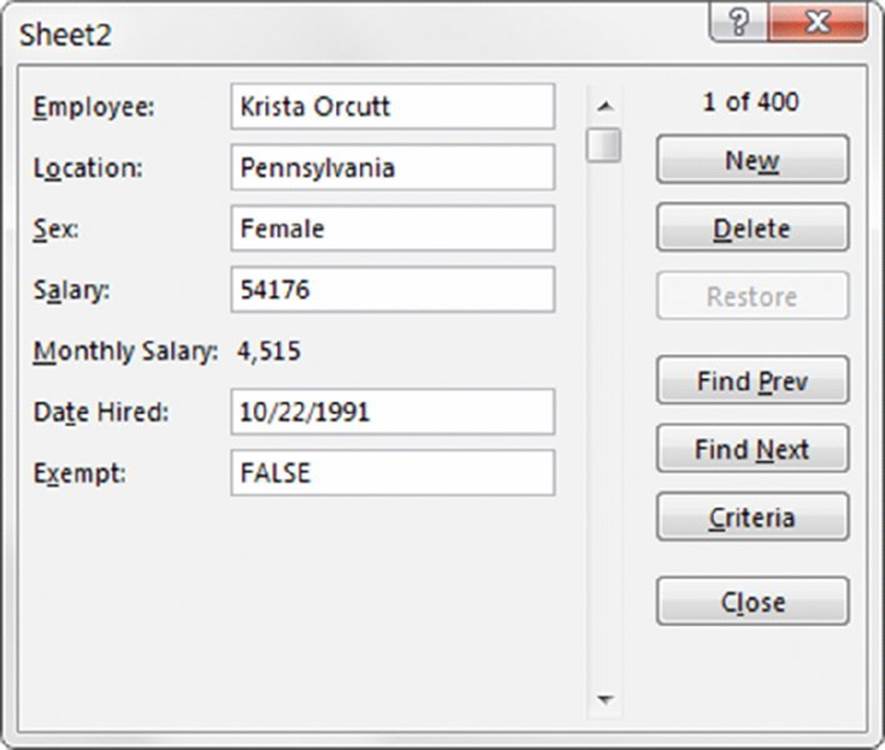
Using a Data form

Excel can display a dialog box to help you work with a list or table. This Data form enables you to enter new data, delete rows, and search for rows that match certain criteria; and it works with either a list or a range that has been designated as a table (choosing the Insert ➜ Tables ➜ Table command).

Unfortunately, the command to access the Data form is not on the Ribbon. To use the Data form, you must add it to your Quick Access toolbar:

1. Right-click the Quick Access toolbar and choose Customize Quick Access Toolbar from the menu that appears.

Excel displays the Quick Access Toolbar tab of the Excel Options dialog box.

2. From the Choose Commands From drop-down list, select Commands Not in the Ribbon.

3. In the list box on the left, select Form.

4. Click the Add button to add the selected command to your Quick Access toolbar.

5. Click OK to close the Excel Options dialog box.

After performing these steps, a new icon appears on your Quick Access toolbar.

Excel’s Data form can be handy (if you like that sort of thing) but is by no means ideal. If you like the idea of using a dialog box to work with data in a table, check out John Walkenbach’s Enhanced Data Form add-in. It offers many advantages over Excel’s Data form. You can download a free copy from the website www.spreadsheetpage.com.

Removing duplicate rows from a table

If data in a table was compiled from multiple sources, the table may contain duplicate items. Most of the time, you want to eliminate the duplicates. In the past, removing duplicate data was essentially a manual task, but it’s easy if the data is in a table.

Start by selecting any cell in your table and then choose Table Tools ➜ Design ➜ Tools ➜ Remove Duplicates. Excel responds with a dialog box like the one shown in Figure 9.5. The dialog box lists all the columns in your table. Place a check mark next to the columns that you want to include in the duplicate search. Most of the time, you’ll want to select all the columns, which is the default. Click OK, and Excel weeds out the duplicate rows and displays a message that tells you how many duplicates it removed.

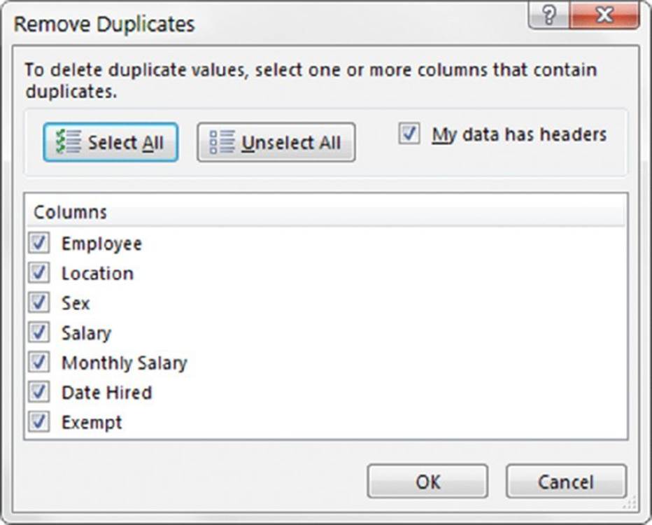
Figure 9.5 Removing duplicate rows from a table is easy.

Unfortunately, Excel does not provide a way for you to review the duplicate records before deleting them. You can, however, use Undo (or press Ctrl+Z) if the result isn’t what you expect.

Tip

If you want to remove duplicates from a list that’s not a table, choose Data ➜ Data Tools ➜ Remove Duplicates.

Warning

Duplicate values are determined by the value displayed in the cell—not necessarily the value stored in the cell. For example, assume that two cells contain the same date. One of the dates is formatted to display as 5/15/2015, and the other is formatted to display as May 15, 2015. When removing duplicates, Excel considers these dates to be different.

Sorting and filtering a table

Each column in the Header row of a table contains a clickable control (a Filter button), which normally displays a downward-pointing arrow. That control, when clicked, displays sorting and filtering options.

Note

You can toggle the display of Filter buttons in a table’s Header row. Choose Table Tools ➜ Design ➜ Table Style Options ➜ Filter Button to display or hide the drop-down arrows.

Figure 9.6 shows a table of real estate listing information after clicking the control for the Date Listed column. If a column is filtered or sorted, the image on the control changes to remind you that the column was used in a filter or sort operation.

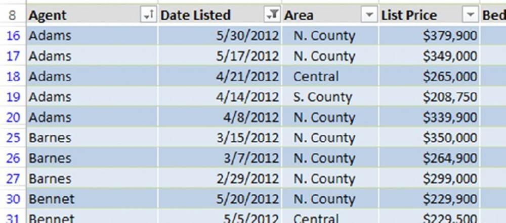
Figure 9.6 Each column in a table contains sorting and filtering options.

On the Web

This workbook, named real estate table.xlsx, is available at this book’s website.

Tip

If you’re working with a list (rather than a table), use Data ➜ Sort & Filter ➜ Filter to add Filter button controls to the top row of your list. This command is a toggle, so you can hide the drop-down arrows by selecting that command again. You can also use Data ➜ Sort & Filter ➜ Filter to hide the drop-down arrows in a table.

Sorting a table

Sorting a table rearranges the rows based on the contents of a particular column. You may want to sort a table to put names in alphabetical order. Or, maybe you want to sort your sales staff by the total sales made.

To sort a table by a particular column, click the drop-down arrow in the column header and choose one of the sort commands. The exact command varies, depending on the type of data in the column. Sort A to Z and Sort Z to A are the options that appear when the columns contain text. The options for columns that contain numeric data or True/False are Sort Smallest to Largest and Sort Largest to Smallest. Columns that contain dates change the options into Sort Oldest to Newest and Sort Newest to Oldest.

You can also select Sort by Color to sort the rows based on the background or text color of the data. This option is relevant only if you’ve overridden the table style colors with custom colors or you’ve used conditional formatting to apply colors based on the cell contents.

Tip

When a column is sorted, the drop-down control in the Header row displays a different graphic to remind you that the table is sorted by that column. If you sort by several columns, only the column most recently sorted displays the sort graphic.

You can sort on any number of columns. The trick is to sort the least significant column first and then proceed until the most significant column is sorted last.

For example, in the real estate listing table (refer to Figure 9.6), you may want the list to be sorted by agent. And within each agent’s group, the rows should be sorted by area. And within each area, the rows should be sorted (descending) by list price. For this type of sort, first sort by the List Price column, then sort by the Area column, and then sort by the Agent column. Figure 9.7 shows the table sorted in this manner.

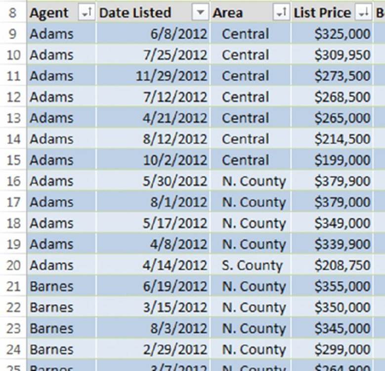
Figure 9.7 A table, after performing a three-column sort.

Another way of performing a multiple-column sort is to use the Sort dialog box. To display this dialog box, choose Home ➜ Editing ➜ Sort & Filter ➜ Custom Sort. Or right-click any cell in the table and choose Sort ➜ Custom Sort from the shortcut menu.

In the Sort dialog box, use the drop-down lists to specify the first search specifications. Note that the searching is opposite of what we described earlier. In this example, you start with Agent. Then click the Add Level button to insert another set of search controls. In this set of controls, specify the sort specifications for the Area column. Then add another level and enter the specifications for the List Price column. Figure 9.8 shows the dialog box after entering the specifications for the three-column sort. This technique produces the same sort as described previously.

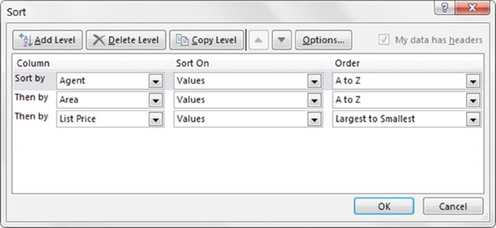
Figure 9.8 Using the Sort dialog box to specify a three-column sort.

Filtering a table

Filtering a table refers to displaying only the rows that meet certain conditions. After you apply a filter, rows that don’t meet the conditions are hidden. Filtering a table lets you focus on a subset of interest.

Note

Excel provides two ways to filter a table. This section discusses standard filtering, which is adequate for most filtering requirements. For more complex filter criteria, you may need to use advanced filtering (discussed later in this chapter).

Using the real estate table, assume that you’re only interested in the data for the N. County area. Click the drop-down control in the Area Row header and remove the check mark from Select All, which deselects everything. Then place a check mark next to N. County (see Figure 9.9). Click OK, and the table will be filtered to display only the listings in the N. County area. Rows for other areas are hidden.

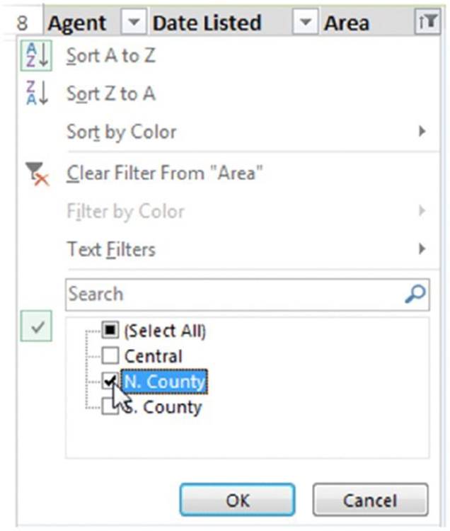
Figure 9.9 Filtering a table to show only the information for N. County.

You can filter by multiple values—for example, filter the table to show only N. County and Central.

You can filter a table using any number of columns. For example, you may want to see only the N. County listings in which the Type is Single Family. Just repeat the operation using the Type column. All tables then display only the rows in which the Area is N. County and the Type is Single Family.

For additional filtering options, select Text Filters (or Number Filters, if the column contains values). The options are fairly self-explanatory, and you have a great deal of flexibility in displaying only the rows that you’re interested in.

In addition, you can right-click a cell and use the Filter command on the shortcut menu. This menu item leads to several additional filtering options. For example, you can filter the table to show only rows that contain the same value as the active cell.

Note

As you may expect, the Total row (if present) is updated to show the total for the visible rows only.

When you copy data in a filtered table, only the visible rows are copied. This filtering makes it easy to copy a subset of a larger table and paste it to another area of your worksheet. Keep in mind that the pasted data is not a table—it’s just a normal range.

Similarly, you can select and delete the visible rows in the table, and the rows hidden by filtering will not be affected.

You cannot, however, unhide rows that are hidden by filtering. For example, if you select all the rows in a table, right-click, and choose Unhide, that command has no effect.

To remove filtering for a column, click the drop-down control in the row Header and select Clear Filter. If you’ve filtered using multiple columns, it may be faster to remove all filters by choosing Home ➜ Editing ➜ Sort & Filter ➜ Clear.

Filtering a table with Slicers

Another way to filter a table is to use one or more Slicers. This method is less flexible but more visually appealing. Slicers are particularly useful when the table will be viewed by novices or those who find the normal filtering techniques too complicated. Slicers are visual, and it’s easy to see exactly what type of filtering is in effect. A disadvantage of Slicers is that they take up a lot of room onscreen.

Note

Slicers for tables was added as a feature in Excel 2013. Slicers for pivot tables were introduced in Excel 2010, but as you may have deduced, they only worked with pivot tables.

To add one or more Slicers, activate any cell in the table and choose Table Tools ➜ Design ➜ Tools ➜ Insert Slicer. Excel responds with a dialog box that displays each header in the table. Place a check mark next to the field(s) that you want to filter. You can create a Slicer for each column, but that’s rarely needed. In most cases, you’ll want to be able to filter the table by only a few fields. Click OK, and Excel creates a Slicer for each field you specified.

Figure 9.10 shows a table with two Slicers. The table is filtered to show only the records for Adams and Jenkins in the Central area.

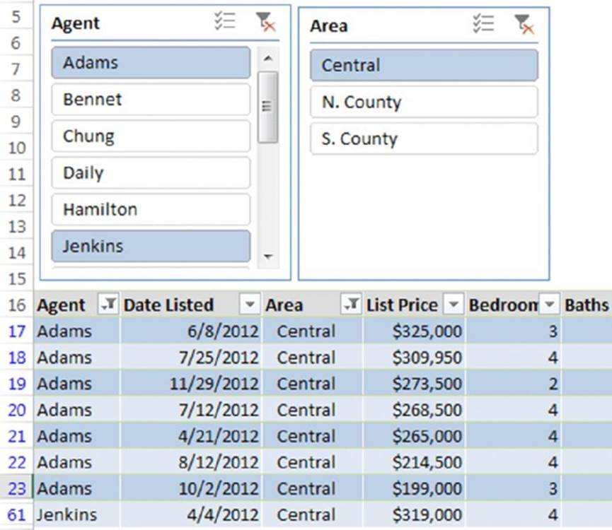
Figure 9.10 The table is filtered by two Slicers.

A Slicer contains a button for every unique item in the field. In the real estate listing example, the Slicer for the Agent field contains 14 buttons because the table has records for 14 different agents.

Note

Slicers may not be appropriate for columns that contain numeric data. For example, the real estate listing table has 78 different values in the List Price column. Therefore, a Slicer for this column would have 78 buttons.

To use a Slicer, just click one of the buttons. The table displays only the rows that correspond to the button. You can also press Ctrl to select multiple buttons and press Shift to select a continuous group of buttons, which would be useful for selecting a range of List Price values.

If your table has more than one Slicer, it’s filtered by the selected buttons in each Slicer. To remove filtering for a particular Slicer, click the icon in the upper-right corner of the Slicer.

Use the tools from the Slicer Tools ➜ Options contextual menu to change the appearance or layout of a Slicer. You have quite a bit of flexibility.

Working with the Total row

The Total row is an optional table element that contains formulas that summarize the information in the columns. Normally, the Total row isn’t displayed. To display the Total row, choose Table Tools ➜ Design ➜ Table Style Options ➜ Total Row. This command is a toggle that turns the Total row on and off.

By default, the Total row displays the sum of the values in a column of numbers. In many cases, you’ll want a different type of summary formula. When you select a cell in the Total row, a drop-down arrow appears, and you can select from a number of other summary formulas (see Figure 9.11):

§ None: No formula.

§ Average: Displays the average of the numbers in the column.

§ Count: Displays the number of entries in the column. (Blank cells are not counted.)

§ Count Numbers: Displays the number of numeric values in the column. (Blank cells, text cells, and error cells are not counted.)

§ Max: Displays the maximum value in the column.

§ Min: Displays the minimum value in the column.

§ Sum: Displays the sum of the values in the column.

§ StdDev: Displays the standard deviation of the values in the column. Standard deviation is a statistical measure of how “spread out” the values are.

§ Var: Displays the variance of the values in the column. Variance is another statistical measure of how “spread out” the values are.

§ More Functions: Displays the Insert Function dialog box so that you can select a function that isn’t in the list.

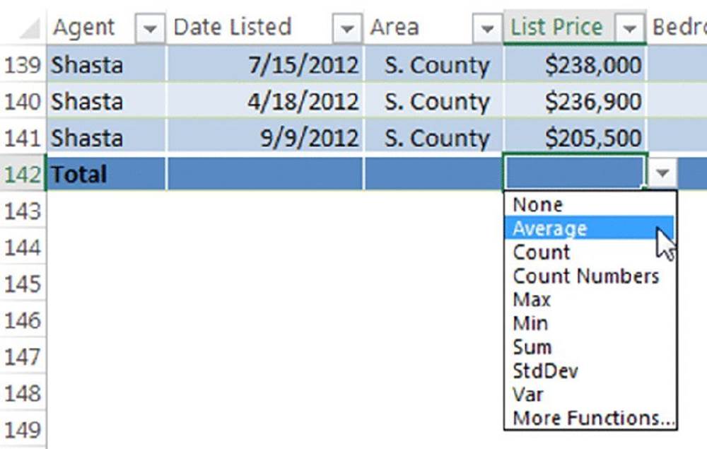
Figure 9.11 Several types of summary functions are available for the Total row.

Using the drop-down list, you can select a summary function for the column. Excel inserts a formula that uses the SUBTOTAL function and refers to the table’s column using a special structured syntax (described later). The first argument of the SUBTOTAL function determines the type of summary displayed. For example, if the first argument is 109, the function displays the sum. You can override the formula inserted by Excel and enter any formula you like in the Total row cell. For more information, see the sidebar “About the SUBTOTAL function.”

Warning

The SUBTOTAL function is one of two functions that ignore data hidden by filtering. (The other is the AGGREGATE function.) If you have other formulas that refer to data in a filtered table, these formulas don’t adjust to use only the visible cells. For example, if you use the SUM function to add the values in column C and some rows are hidden because of filtering, the formula continues to show the sum for all the values in column C—not just those in the visible rows.

Warning

If you have a formula that refers to a value in the Total row of a table, the formula returns an error if you hide the Total row. However, if you make the Total row visible again, the formula works as it should.

About the SUBTOTAL function

The SUBTOTAL function is versatile, but it’s also one of the most confusing functions in Excel’s arsenal. First of all, it has a misleading name because it does a lot more than addition. The first argument for this function requires an arbitrary (and impossible to remember) number that determines the type of result that’s returned. Fortunately, the Excel Formula AutoComplete feature helps you insert these numbers.

In addition, the SUBTOTAL function was enhanced in Excel 2003 with an increase in the number of choices for its first argument, which opens the door to compatibility problems if you share your workbook with someone who uses an earlier version of Excel.

The first argument for the SUBTOTAL function determines the actual function used. For example, when the first argument is 1, the SUBTOTAL function works like the AVERAGE function. When you enter a formula that uses the SUBTOTAL function, the Formula AutoComplete feature guides you through the arguments, so you never have to memorize the numbers.

When the first argument is greater than 100, the SUBTOTAL function behaves a bit differently. Specifically, it does not include data in rows that were hidden manually. When the first argument is less than 100, the SUBTOTAL function includes data in rows that were hidden manually but excludes data in rows that were hidden as a result of filtering or using an outline.

To add to the confusion, a manually hidden row is not always treated the same. If a row is manually hidden in a range that already contains rows hidden via a filter, Excel treats the manually hidden rows as filtered rows. After a filter is applied, Excel can’t seem to tell the difference between filtered rows and manually hidden rows. The SUBTOTAL function with a first argument over 100 behaves the same as those with a first argument under 100, and removing the filter shows all rows—even the manually hidden ones.

Another interesting characteristic of the SUBTOTAL function is its ability to produce an accurate grand total. It does this by ignoring any cells that already contain a formula with SUBTOTAL in them. For a demonstration of this ability, see the “Inserting Subtotals” section later in this chapter.

Using formulas within a table

Adding a Total row to a table is an easy way to summarize the values in a table column. In many cases, you’ll want to use formulas within a table. For example, in the table shown in Figure 9.12, you might want to add a column that shows the difference between the Actual and the Projected amounts. As you’ll see, Excel makes this easy when the data is in a table.

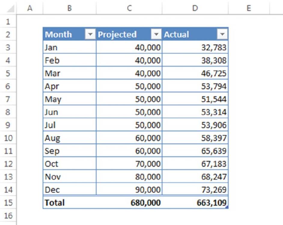
Figure 9.12 Adding a calculated column to this table is easy.

On the Web

This workbook, named table formulas.xlsx, is available at this book’s website.

To add a column that calculates the difference between the Actual and Projected columns, follow these steps:

1. Activate cell E2 and type Difference for the column header.

2. Excel automatically expands the table to include a new column.

3. Move to cell E3 and type an equal sign to signify the beginning of a formula.

4. Press the left arrow, and Excel displays =[@Actual], which is the column heading in the Formula bar.

5. Type a minus sign and then press the left arrow twice. Excel displays =[@Actual]-[@Projected] in your formula.

6. Press Enter to end the formula.

Excel copies the formula to all rows in the table.

Figure 9.13 shows the table with the new calculated column.

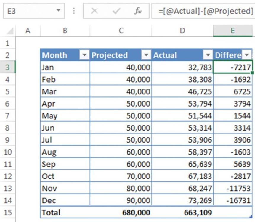
Figure 9.13 The Difference column contains a formula.

If you examine the table, you’ll find this formula for all cells in the Difference column:

=[@Actual]-[@Projected]

Note

The @ symbol that precedes the column header represents “this row” (the row that contains the formula). So each formula in column E calculates “this row’s Actual value minus this row’s Projected value.”

The syntax is a bit different if a column header contains spaces or nonalphanumeric characters such as a pound sign, an asterisk, and so on). In such a case, Excel encloses the column header text in brackets (not quote marks). For example, if the column C header was Projected Income, the formula would appear as follows:

=[@Actual]-[@[Projected Income]]

Some symbols in a column header (such as a square bracket) require the use of an apostrophe as an escape character. It is usually much simpler to create table formulas by pointing and let Excel handle the syntax details.

Keep in mind that we didn’t define names in this worksheet. The formula uses table references that are based on the column names. If you change the text in a column header, any formulas that refer to that data update automatically. That’s an example of how working with a table is easier than working with a regular list.

Although we entered the formula into the first data row of the table, that’s not necessary. We could have put that formula in any cell in column D. Any time you enter a formula into any cell in an empty table column, it will automatically fill all the cells in that column. And if you need to edit the formula, edit the copy in any row, and Excel automatically copies the edited formula to the other cells in the column.

The preceding steps use the pointing technique to create the formula. Alternatively, you can enter the formula manually using standard cell references. For example, you can enter the following formula in cell E3:

=D3-C3

If you type the formulas using cell references, Excel still copies the formula to the other cells automatically; it just doesn’t use the column headings.

Tip

When Excel inserts a calculated column formula, it also displays an icon. Click the icon to display some options, one of which is Stop Automatically Creating Calculated Columns. Select this option if you prefer to do your own copying within a column.

Referencing data in a table

The preceding section describes how to create a column of formulas within a table—often called a calculated column. What about formulas outside a table that refer to data inside a table? You can take advantage of the structured table referencing that uses the table name, column headers, and other table elements. You don’t need to create names for these items.

The table itself has a name that was assigned automatically when you created the table (for example, Table1), and you can refer to data within the table by using the column header text.

You can, of course, use standard cell references to refer to data in a table, but the structured table referencing has a distinct advantage: the names adjust automatically if the table size changes by adding or deleting rows.

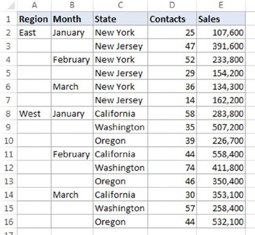
Figure 9.14 shows a simple table that contains regional sales information. Excel named this table Table2 when it was created because it was the second table in the workbook. To calculate the sum of all the values in the table, use this formula:

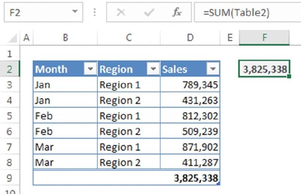
Figure 9.14 This table shows sales by month and by region.

=SUM(Table2)

This formula always returns the sum of all the data, even if rows or columns are added or deleted. And if you change the name of the table, Excel adjusts all formulas that refer to that table automatically. For example, if you rename Table1 to be Q1Data, the preceding formula changes to this:

=SUM(Q1Data)

Tip

To change the name of a table, select any cell in the table and use the Table Name box of the Table Tools ➜ Design ➜ Properties group. Or you can use the Name Manager to change the name of a table (Formulas ➜ Defined Names ➜ Name Manager).

Most of the time, your formulas will refer to a specific column in the table rather than the entire table. The following formula returns the sum of the data in the Sales column:

=SUM(Table2[Sales])

Notice that the column name is enclosed in square brackets. Again, the formula adjusts automatically if you change the text in the column heading.

Warning

Keep in mind that the preceding formula does not adjust if table rows are hidden as a result of filtering. SUBTOTAL and AGGREGATE are the only functions that change their result to ignore hidden rows. To sum the Sales column and ignore filtered rows, use either of the following formulas:

=SUBTOTAL(109,Table2[Sales])

=AGGREGATE(9,1,Table2[Sales])

Excel provides some helpful assistance when you create a formula that refers to data within a table. Figure 9.15 shows the Formula AutoComplete feature helping create a formula by showing a list of the elements in the table. The list appeared after we typed the left square bracket.

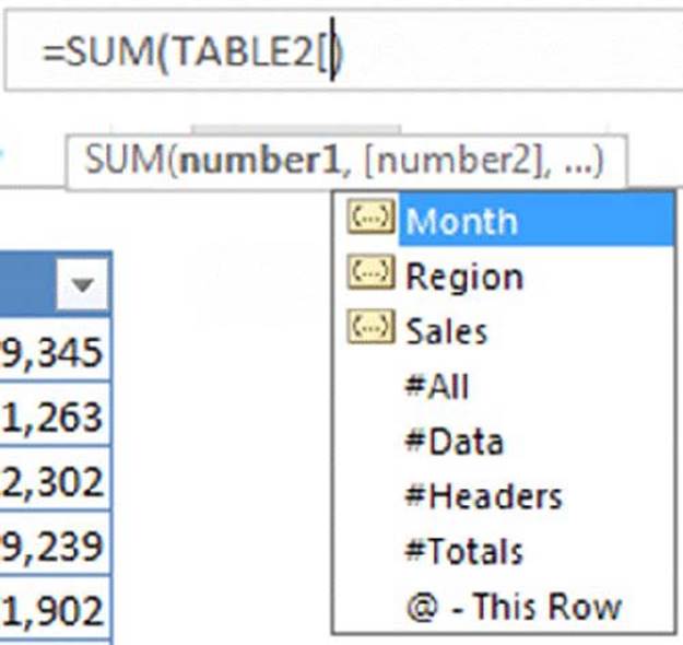
Figure 9.15 The Formula AutoComplete feature is useful when creating a formula that refers to data in a table.

Here’s another example that returns the sum of the January sales:

=SUMIF(Table2[Month],"Jan",Table2[Sales])

Cross-Ref

For an explanation of the SUMIF worksheet function, refer to Chapter 7, “Counting and Summing Techniques.”

Using this structured table syntax is optional—you can use actual range references if you like. For example, the following formula returns the same result as the preceding one:

=SUMIF(B3:B8,"Jan",D3:D8)

To refer to a cell in the Total row of a table, use a formula like this:

=Table2[[#Totals],[Sales]]

This formula returns the value in the Total row of the Sales column in Table2. If the Total row in Table2 is not displayed, the preceding formula returns a #REF error.

To count the total number of rows in Table2, use the following formula:

=ROWS(Table2[#All])

The preceding formula counts all rows, including the Header row, Total row, and hidden rows.

To count only the data rows (including hidden rows), use a formula like this:

=ROWS(Table2[#Data])

To count only the visible data rows, use the SUBTOTAL or AGGREGATE function. For example, you can use either of these formulas:

=SUBTOTAL(103,Table2[Region])

=AGGREGATE(3,5,Table2[Region])

Because the formula is counting visible rows, you can use any column header in the preceding formula.

A formula that’s not in the table but is in the same row as a table can use an @ reference to refer to table data that is in the same row. For example, assume the following formula is in row 3, in a column outside Table2. The formula returns the value in row 3 of the Sales column in Table2:

= Table2[@Sales])

You can also combine row and column references by nesting brackets and including multiple references separated by commas. The following example returns Sales from the current row divided by the total sales:

=Table2[@Sales]/Table2[[#Totals],[Sales]]

A formula like the preceding one is much easier to create if you use the pointing method.

Table 9.1 summarizes the row identifiers for table references and describes which ranges they represent.

Table 9.1 Table Row References

Filling in the gaps

When you import data, you can end up with a worksheet that looks something like the one in the accompanying figure. In this example, an entry in column A applies to several rows of data. If you sort such a range, you can end up with a mess, and you won’t be able to tell who sold what.

When you have a small range, you can type the missing cell values manually. If your list has hundreds of rows, though, you need a better way of filling in those cell values. Here’s how:

1. Select the range (A1:A16 in this example).

2. Choose Home ➜ Editing ➜ Find & Select ➜ Go To Special to display the Go To Special dialog box.

3. In the Go To Special dialog box, select the Blanks option.

4. Click OK to close the Go To Special dialog box.

5. In the Formula bar, type =, followed by the address of the first cell with an entry in the column (=A2 in this example), and then press Ctrl+Enter to copy that formula to all selected cells.

6. Reselect the range from step 1 and press Ctrl+C.

7. Choose Home ➜ Clipboard ➜ Paste Values (V).

Each blank cell in the column is filled with data from above.

Converting a table to a list

In some cases, you may need to convert a table back to a normal list. For example, you may need to share your workbook with someone who uses an older version of Excel. Or, maybe you’d like the use the Custom Views feature (which is disabled when the workbook contains a table). To convert a table to a normal list, just select a cell in the table and choose Table Tools ➜ Design ➜ Tools ➜ Convert To Range. The table style formatting remains intact, but the range no longer functions as a table.

Formulas inside and outside the table that use structured table references are converted, so they use range addresses rather than table items.

Using Advanced Filtering

In many cases, standard filtering (as we described previously in this chapter) does the job just fine. If you run up against its limitations, you need to use advanced filtering. Advanced filtering is much more flexible than standard filtering, but it takes a bit of upfront work to use it. Advanced filtering provides you with the following capabilities:

§ You can specify more complex filtering criteria.

§ You can specify computed filtering criteria.

§ You can automatically extract a copy of the rows that meet the criteria and place it in another location.

You can use advanced filtering with a list or with a table.

The examples in this section use a real estate listing list (shown in Figure 9.16), which has 125 rows and 10 columns. This list contains an assortment of data types: value, text string, logical, and date. The list occupies the range A8:J133. (Rows above the table are used for the criteria range.)

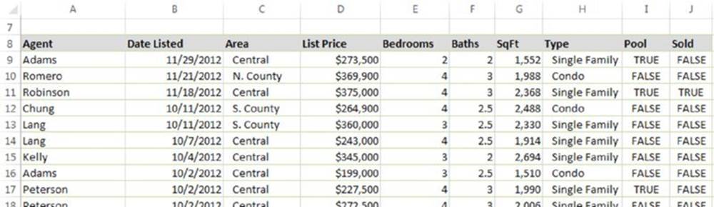
Figure 9.16 This real estate listing table is used to demonstrate advanced filtering.

On the Web

This workbook, named real estate list.xlsx, is available at this book’s website.

Setting up a criteria range

Before you can use the advanced filtering feature, you must set up a criteria range, which is a range on a worksheet that conforms to certain requirements. The criteria range holds the information that Excel uses to filter the table. The criteria range must conform to the following specifications:

§ It must consist of at least two rows, and the first row must contain some or all of the column names from the table. An exception to this is when you use computed criteria. Computed criteria can use an empty Header cell. (See the “Specifying computed criteria” section later in this chapter.)

§ The other rows of the criteria range contain your filtering criteria.

You can put the criteria range anywhere in the worksheet or even in a different worksheet. However, you should avoid putting the criteria range in rows that are occupied by the list or table. Because Excel may hide some of these rows when filtering, you may find that your criteria range is no longer visible after filtering. Therefore, you should generally place the criteria range above or below the table.

Figure 9.17 shows a criteria range in A1:B2, located above the list that it uses. Notice that the criteria range does not include all the field names from the table. You can include only the field names for fields that you use in the selection criteria.

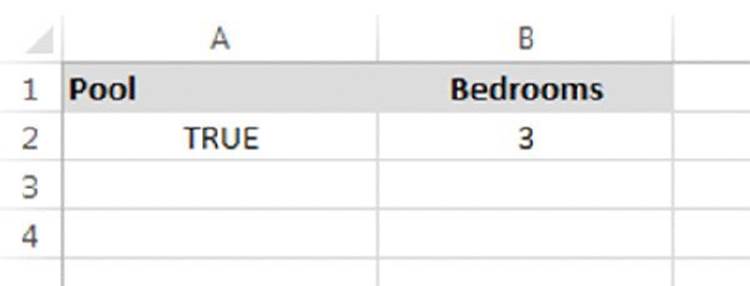
Figure 9.17 A criteria range for advanced filtering.

In this example, the criteria range has only one row of criteria. The fields in each row of the criteria range are joined with an AND operator. Therefore, after applying the advanced filter, the list shows only the rows in which the Bedrooms column is 3 and the Pool column is TRUE. In other words, it shows only the listings for three-bedroom homes with a pool.

You may find specifying criteria in the criteria range a bit tricky. We discuss this topic in detail later in this chapter in the section “Specifying Advanced Filter Criteria.”

Applying an advanced filter

To perform the advanced filtering:

1. Ensure that you’ve set up a criteria range.

2. Choose Data ➜ Sort & Filter ➜ Advanced.

Excel displays the Advanced Filter dialog box, as shown in Figure 9.18.

3. Excel guesses your database range if the active cell is within or adjacent to a block of data, but you can change it if necessary.

4. Specify the criteria range.

If you happen to have a named range with the name Criteria, Excel will insert that range in the Criteria Range field—you can also change this range if you like.

5. To filter the database in place (that is, to hide rows that don’t qualify), select the option labeled Filter the List, In-Place.

If you select Copy to Another Location, you need to specify a range in the Copy To field. Specifying the upper-left cell of an empty range will do.

6. Click OK, and Excel filters the table by the criteria that you specify.

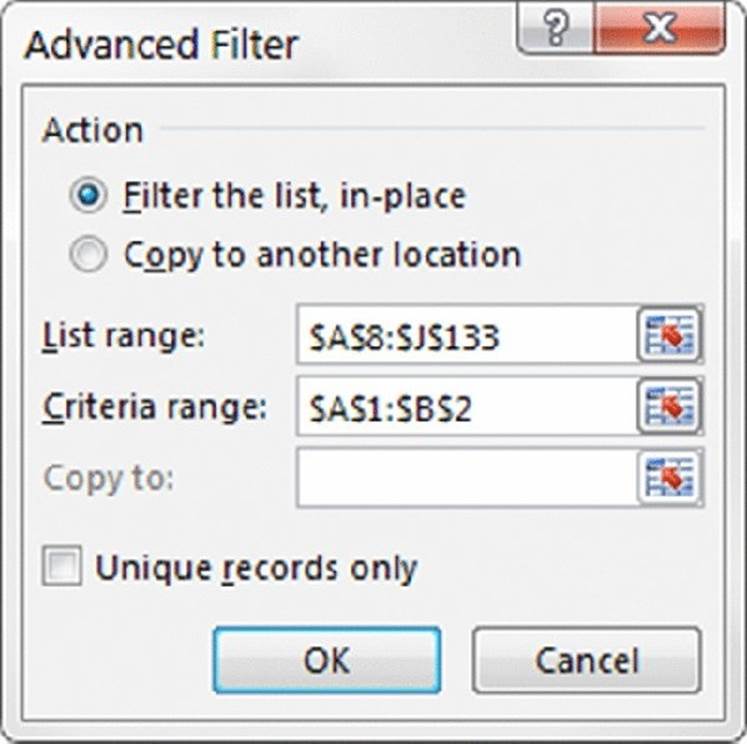
Figure 9.18 The Advanced Filter dialog box.

Figure 9.19 shows the list after applying the advanced filter that displays three-bedroom homes with a pool.

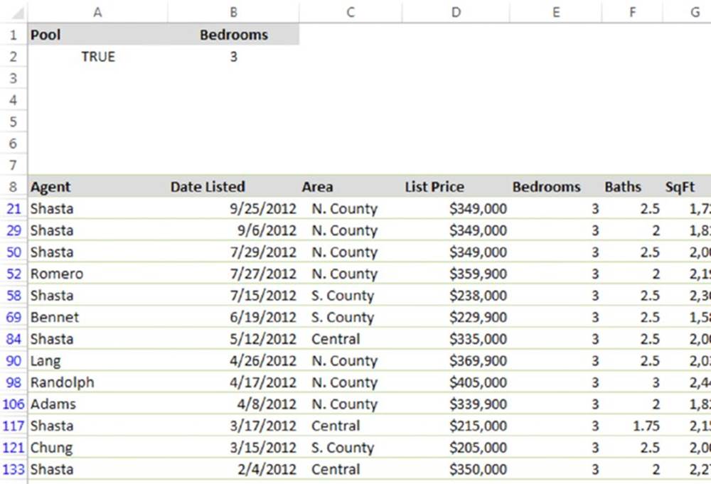
Figure 9.19 The result of applying an advanced filter.

Tip

When you select the Copy to Another Location option, you can specify which columns to include in the copy. Before displaying the Advanced Filter dialog box, copy the desired field labels to the first row of the area where you plan to paste the filtered rows. In the Advanced Filter dialog box, specify a reference to the copied column labels in the Copy To field. The copied rows then include only the columns for which you copied the labels.

Clearing an advanced filter

When you apply an advanced filter, Excel hides all rows that don’t meet the criteria you specified. To clear the advanced filter and display all rows, choose Data ➜ Sort & Filter ➜ Clear.

Specifying Advanced Filter Criteria

The key to using advanced filtering is knowing how to set up the criteria range, which is the focus of the sections that follow. You have a great deal of flexibility, but some of the options are not exactly intuitive. Here, you’ll find plenty of examples to help you understand how to create a criteria range that extracts the information you need.

Note

The use of a separate criteria range for advanced filtering originated with the first version of Lotus 1-2-3, more than 30 years ago. Excel adapted this method, and it has never been changed, despite the fact that specifying advanced filtering criteria remains one of the most confusing aspects of Excel. Fortunately, however, Excel’s standard filtering is sufficient for most needs.

Specifying a single criterion

The examples in this section use a single-selection criterion. In other words, the contents of a single field determine the record selection.

Note

You also can use standard filtering to perform this type of filtering.

To select only the records that contain a specific value in a specific field, enter the field name in the first row of the criteria range and the value to match in the second row.

Note that the criteria range does not need to include all the fields from the database. If you work with different sets of criteria, you may find it more convenient to list all the field names in the first row of your criteria range.

Using comparison operators

You can use comparison operators to refine your record selection. For example, you can select records based on any of the following single criteria:

§ Homes with at least four bedrooms

§ Homes with square footage less than 2,000

§ Homes with a list price of no more than $250,000

To select the records that describe homes that have at least four bedrooms, type Bedrooms in cell A1 and then type >=4 in cell A2 of the criterion range.

Table 9.2 lists the comparison operators that you can use with text or value criteria. If you don’t use a comparison operator, Excel assumes the equal sign operator (=).

Table 9.2 Comparison Operators

Using wildcard characters

Criteria that use text also can make use of two wildcard characters: an asterisk (*) matches any number of characters; a question mark (?) matches any single character.

Table 9.3 shows examples of criteria that use text. Some of these are a bit counterintuitive. For example, to select records that match a single character, you must enter the criterion as a formula (refer to the last entry in the table).

Table 9.3 Examples of Text Criteria

Note

The text comparisons are not case sensitive. For example, se* matches Seligman, seller, and SEC.

Specifying multiple criteria

Often, you may want to select records based on criteria that use more than one field or multiple values within a single field. These selection criteria involve logical OR or AND comparisons. Here are a few examples of the types of multiple criteria that you can apply to the real estate database:

§ A list price less than $250,000, and square footage of at least 2,000

§ A single-family home with a pool

§ At least four bedrooms, at least three bathrooms, and square footage less than 3,000

§ A home that has been listed for no more than two months, with a list price greater than $300,000

§ A condominium with square footage between 1,000 and 1,500

§ A single-family home listed in the month of March

To join criteria with an AND operator, use multiple columns in the criteria range. Figure 9.20 shows a criteria range that filters records to show those with at least four bedrooms, more than 3,000 square feet, a pool, and a list price of $390,000 or less.

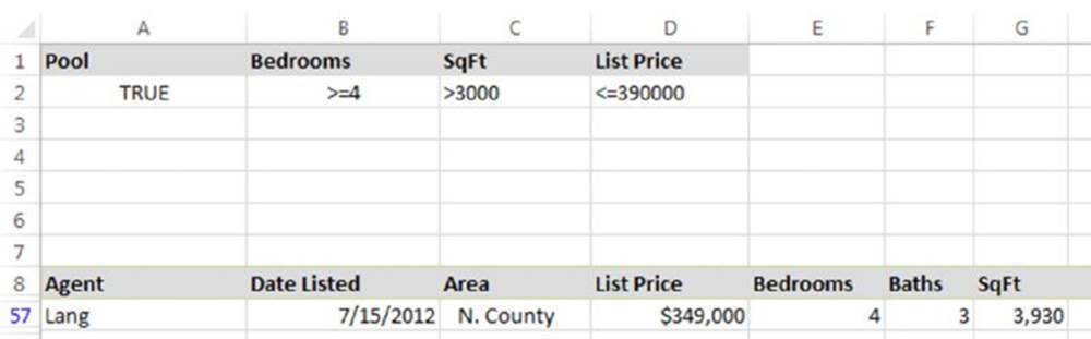
Figure 9.20 This criteria range uses multiple columns that select records using a logical AND operation.

Figure 9.21 shows another example. This criteria range displays listings from the month of August 2012. Notice that the column name (Date Listed) appears twice in the criteria range. The criteria selects the records in which the Date Listed date is greater than or equal to August 1, and the Date Listed date is less than or equal to August 31.

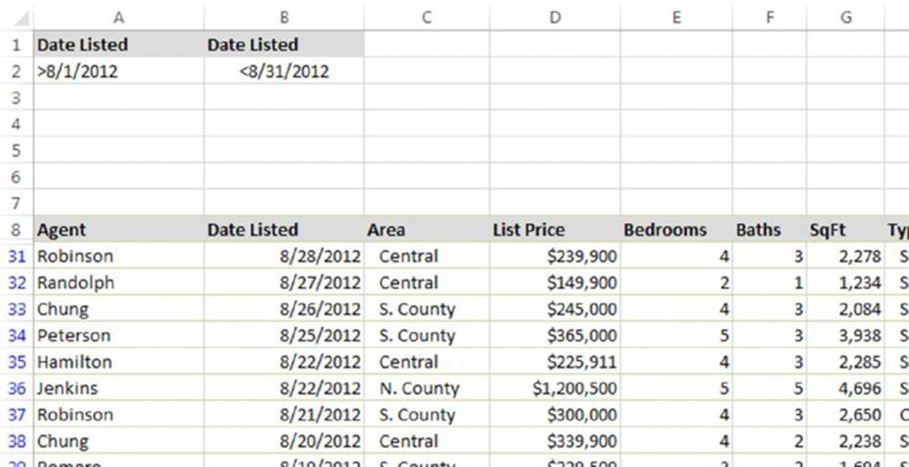
Figure 9.21 This criteria range selects records that describe properties that were listed in the month of August.

Warning

The date selection criteria may not work properly for systems that don’t use the U.S. date formats. To ensure compatibility with different date systems, use the DATE function to define such criteria, as in the following formulas:

=">="&DATE(2012,8,1)

="<="&DATE(2012,8,31)

To join criteria with a logical OR operator, use more than one row in the criteria range. A criteria range can have any number of rows, each of which joins with the others via an OR operator. Figure 9.22 shows a criteria range (A1:D3) with two rows of criteria.

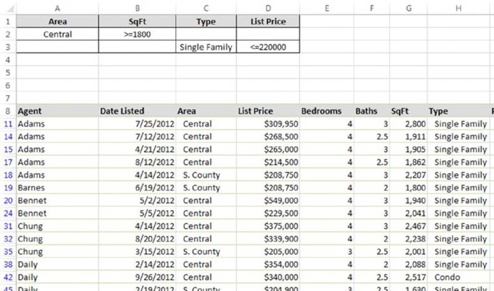
Figure 9.22 This criteria range has two sets of criteria, each of which is in a separate row.

In this example, the filtered table shows the rows that meet either of the following conditions:

§ A property with a square footage of at least 1,800, in the Central area

or

§ A single-family home of any size, priced at $220,000 or less, in any area

Note

This is an example of the type of filtering that you cannot perform by using standard (non-advanced) filtering.

Specifying computed criteria

Using computed criteria can make filtering even more powerful. Computed criteria filter the table based on one or more calculations. For example, you can specify computed criteria that display only the rows in which the List Price (column D) is greater than average.

=D9>AVERAGE(D:D)

Notice that this formula uses a reference to cell D9, the first data cell in the List Price column. Also, when you use computed criteria, the cell above it must not contain a field name. You can leave that cell blank or provide a descriptive label, such as Above Average. The formula will return a value, but that value is meaningless.

By the way, you can also use a standard filter to display data that’s above (or below) average.

The next example displays the rows in which the listing has a pool and the price per square foot is less than $100. Cell D9 is the first data cell in the List Price column, and cell G9 is the first data cell in the SqFt column. In Figure 9.23, the computed criteria formula is

Figure 9.23 Using computed criteria with advanced filtering.

=(D9/G9)<100

Here is another example of a computed criteria formula. This formula displays the records listed within the past 60 days:

=B9>TODAY()-60

Keep the following points in mind when using computed criteria:

§ Computed criteria formulas are always logical formulas: they must return either TRUE or FALSE. However, the value that’s returned is irrelevant.

§ When referring to columns, use a reference to the cell in the first data row in the field of interest (not a reference to the cell that contains the field name).

§ When you use computed criteria, do not use an existing field label in your criteria range. A computed criterion essentially computes a new field for the table. Therefore, you must supply a new field name in the first row of the criteria range. Or, if you prefer, you can simply leave the field name cell blank.

§ You can use any number of computed criteria and mix and match them with noncomputed criteria.

§ If your computed formula refers to a value outside the table, use an absolute reference rather than a relative reference. For example, use $C$1 rather than C1.

§ In many cases, you may find it easier to add a new calculated column to your list or table and avoid using computed criteria.

Using Database Functions

To create formulas that return results based on a criteria range, use Excel’s database worksheet functions. All these functions begin with the letter D, and they are listed in the Database category of the Insert Function dialog box.

Table 9.4 lists Excel’s database functions. Each of these functions operates on a single field in the database.

Table 9.4 Excel Database Worksheet Functions

All the database functions require a separate criteria range, which is specified as the last argument for the function. The database functions use the same type of criteria range as discussed earlier in the “Specifying Advanced Filter Criteria” section (see Figure 9.24).

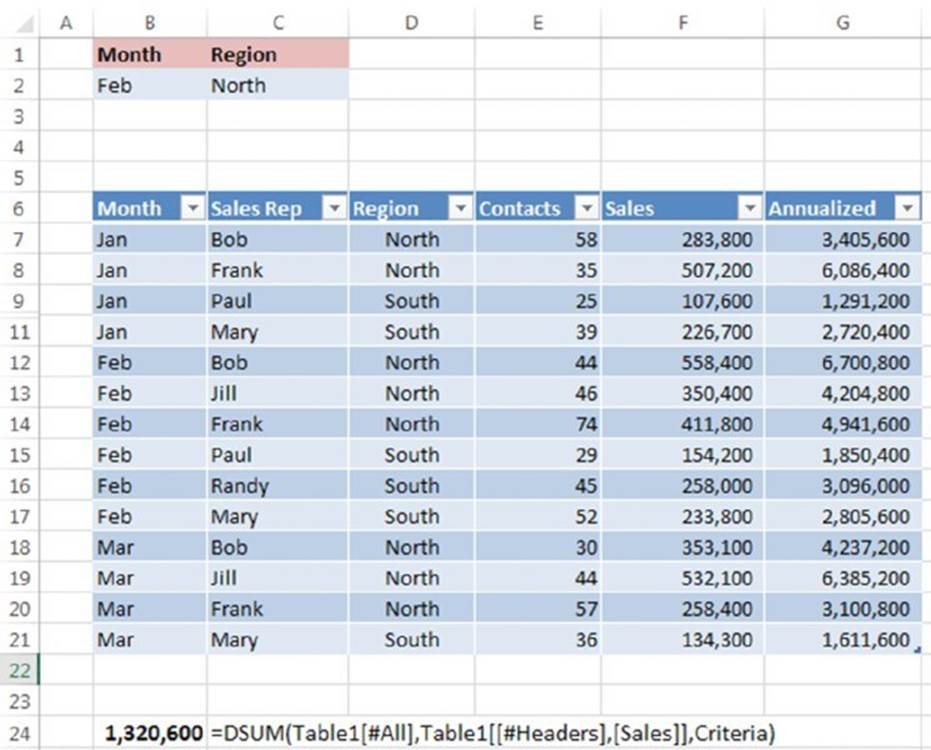
Figure 9.24 Using the DSUM function to sum a table using a criteria range.

The formula in cell B24, which follows, uses the DSUM function to calculate the sum of values in a table that meet certain criteria. Specifically, the formula returns the sum of the Sales column for records in which the Month is Feb and the Region is North.

=DSUM(B6:G21,F6,B1:C2)

In this case, B6:G21 is the entire table, F6 is the column heading for Sales, and B1:C2 is the criteria range.

This alternative version of the formula uses structured table references:

=DSUM(Table1[#All],Table1[[#Headers],[Sales]],B1:C2)

On the Web

This workbook is available at this book’s website. The filename is database formulas .xlsx.

Note

You may find it cumbersome to set up a criteria range every time you need to use a database function. Fortunately, Excel provides some alternative ways to perform conditional sums and counts. See Chapter 7 for examples that use SUMIF, COUNTIF, and various other techniques.

If you’re an array formula aficionado, you might be tempted to use a literal array in place of the criteria range. In theory, the following array formula should work (and would eliminate the need for a separate criteria range). Unfortunately, the database functions do not support arrays, and this formula simply returns a #VALUE! error.

=DSUM(B6:G21,F6, {"Month","Region";"Feb","North"})

Inserting Subtotals

Excel’s Data ➜ Outline ➜ Subtotal command is a handy tool that inserts formulas into a list automatically. These formulas use the SUBTOTAL function. To use this feature, your list must be sorted because the formulas are inserted whenever the value in a specified column changes. For more information about the SUBTOTAL function, refer to the sidebar, “About the SUBTOTAL function,” earlier in this chapter.

Note

When a table is selected, the Data ➜ Outline ➜ Subtotal command is not available. Therefore, this section applies only to lists. If your data is in a table and you need to insert subtotals automatically, convert the table to a range by using Table Tools ➜ Design ➜ Tools ➜ Convert To Range. After you insert the subtotals, you can convert the range back to a table by using Insert ➜ Tables ➜ Table.

Figure 9.25 shows an example of a list that’s appropriate for subtotals. This list is sorted by the Month field, and the Region field is sorted within months.

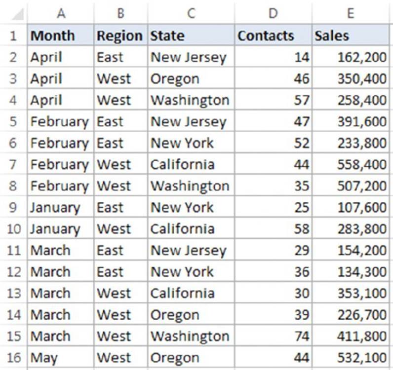
Figure 9.25 This list is a good candidate for subtotals, which are inserted at each change of the month.

On the Web

This workbook, named nested subtotals.xlsx, is available at this book’s website.

To insert subtotal formulas into a list automatically, activate any cell in the range and choose Data ➜ Outline ➜ Subtotal. You will see the Subtotal dialog box, similar to the one shown in Figure 9.26.

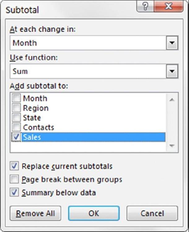
Figure 9.26 The Subtotal dialog box automatically inserts subtotal formulas into a sorted table.

The Subtotal dialog box offers the following choices:

§ At Each Change In: This drop-down list displays all the fields in your table. You must have sorted the list by the field that you choose.

§ Use Function: Choose from 11 functions. (Sum is the default.)

§ Add Subtotal To: This list box shows all the fields in your table. Place a check mark next to the field or fields that you want to subtotal.

§ Replace Current Subtotals: If checked, Excel removes any existing subtotal formulas and replaces them with the new subtotals.

§ Page Break Between Groups: If checked, Excel inserts a manual page break after each subtotal.

§ Summary Below Data: If checked, Excel places the subtotals below the data (the default). Otherwise, the subtotal formulas appear above the data.

§ Remove All: This button removes all subtotal formulas in the list.

When you click OK, Excel analyzes the database and inserts formulas as specified—it even creates an outline for you. Figure 9.27 shows a worksheet after adding subtotals that summarize by month. You can, of course, use the SUBTOTAL function in formulas that you create manually. Using the Data ➜ Outline ➜ Subtotals command is usually easier.

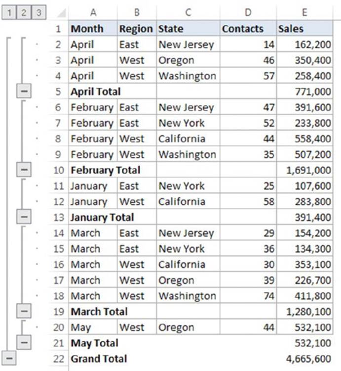
Figure 9.27 Excel adds the subtotal formulas automatically and creates an outline.

All the formulas use the SUBTOTAL worksheet function. For example, the formula in cell E20 (Grand Total) is as follows:

=SUBTOTAL(9,E2:E18)

Although this formula refers to other cells that contain a SUBTOTAL formula, those cells are ignored, to avoid double-counting.

You can use the outline controls to adjust the level of detail shown. Figure 9.28, for example, shows only the summary rows from the subtotaled table. These rows contain the SUBTOTAL formulas.

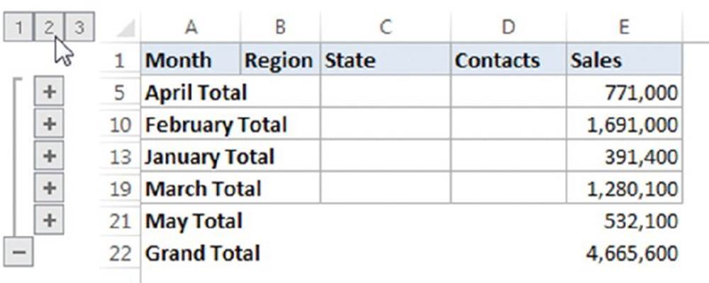
Figure 9.28 Use the outline controls to hide the detail and display only the summary rows.

Note

In most cases, using a pivot table to summarize data is a better choice. Pivot tables are much more flexible, and formulas aren’t required. Figure 9.29 shows a pivot table created from the data. See Chapter 18, “Pivot Tables,” for more information about pivot tables.

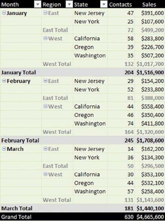
Figure 9.29 Use a pivot table to summarize data. Formulas are not required.