My Excel 2016 (2016)
1. Understanding the Microsoft Excel Interface
In this chapter, you’ll learn some basic Excel terminology and functionality. The topics in this chapter include the following:
→ Identifying parts of the Excel window
→ Customizing the ribbon and QAT
→ Viewing sheets
→ Selecting a range of cells
If you already know how to add a custom tab to the ribbon or select cell D28, then you’ve probably spent some time using Excel. However, if what you’ve just read makes little sense to you, then this chapter is especially for you. This chapter explains the basic parts of the Microsoft Excel window, how to use them, and the terminology used to refer to them. It also shows you how to customize the interface, navigate around a sheet, and select a range of cells.
Identifying Parts of the Excel Window
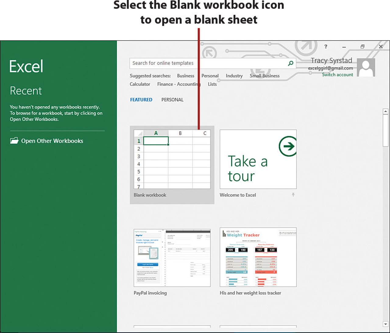
When you open Excel 2016 the first time, you see icons for various templates. Chapter 2, “Working with Workbooks and Templates,” covers templates in more depth. For now, click the Blank workbook icon to open a blank sheet.
Not Seeing the Templates Window
If you don’t see the templates window, a previous user changed the settings to turn off the Start screen. Instead, when you open Excel, you’ll go straight to a blank workbook.
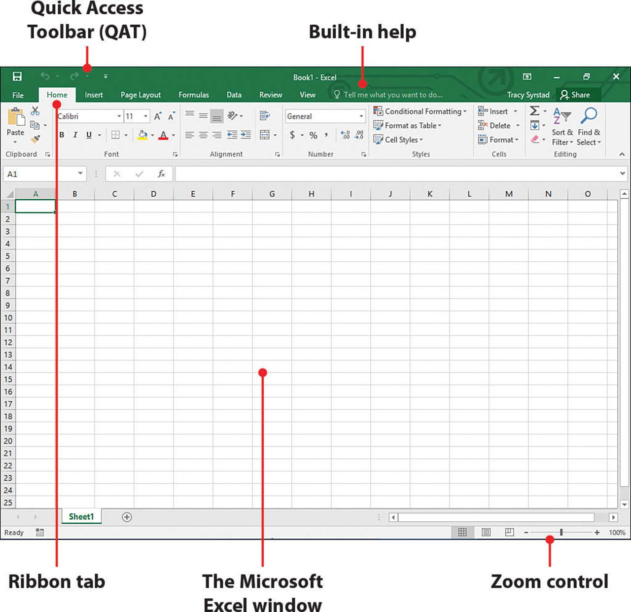
The Excel application window has many parts to it, such as the ribbon, row headings, column headings, and cells. Following are descriptions of the various parts we’ll be interacting with in this book:
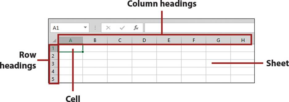
• The big grid taking up most of the Excel window is the sheet, also known as a worksheet or spreadsheet.
• Right above the grid are letters known as column headings. Down the left side of the grid are numbers, also known as row headings.
• An intersection of a column and row is a cell. Each cell has an address made up of the column letter then the row number that intersect at the cell. Multiple cells selected together are commonly known as a range.
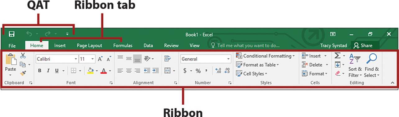
• The ribbon is where you choose what you want to do on your sheet, such as formatting text or inserting a chart. See the section “Making Selections from the Ribbon” for information on the different types of controls on the ribbon. As you use Excel, you’ll notice new tabs in the ribbon appearing, depending on what you’re doing in the sheet area, such as working with a pivot table. These tabs are “context sensitive”—that is, they appear only when they are useful. Other times, they stay out of your way.
It’s Not All Good: My Ribbon Doesn’t Match Yours
The ribbon has nice big buttons on it, but it doesn’t fit well on small screens or low-resolution monitors. To compensate, the ribbon will automatically resize the buttons, but this also gets rid of the labels, leaving only the icons. When the screen is very narrow, entire groups of commands collapse, so you might need to click a group button to see the icons. Throughout this book, you might notice the ribbon in the images doesn’t match yours. In those cases, look for a matching icon.
• The Quick Access Toolbar, also known as the QAT, is always visible, even when the ribbon is minimized. However, unlike in the ribbon, the commands that display in the QAT don’t depend on what you are doing in Excel.
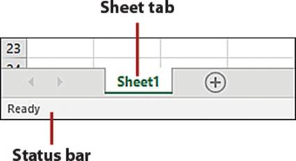
• The status bar has many uses. It holds zoom and page view controls, it lets you know if calculations need to be updated, and it can provide information, such as the sum or average, on a selected range.
• Every sheet in a workbook has a sheet tab. Clicking the tab is how you move between sheets.
Using the Built-in Help
The help interface in Excel provides assistance in three ways. You can use it to jump to a specific command or search Microsoft’s online help system. It can also return more information on any topic from the Internet.
Perform a Search
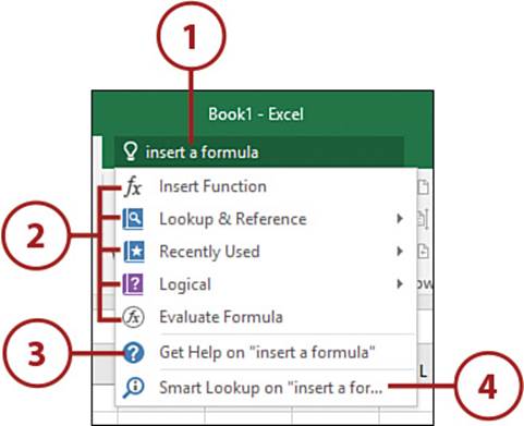
As you enter your search criteria, Excel updates a drop-down of possible matches. The drop-down list is broken into three parts: Excel commands, a Get Help link, and Smart Lookup to run an online search.
1. Click the Tell Me search box and type the search phrase.
2. Select an Excel command. A dialog box might open, a formula might be inserted into a cell, cell formatting changed, or something else, depending on what the command is.
Or
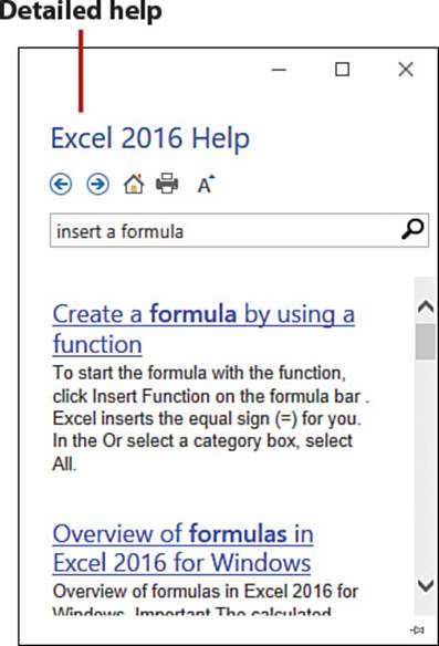
3. Select Get Help to open a new window with information from Microsoft’s online help files.
Or
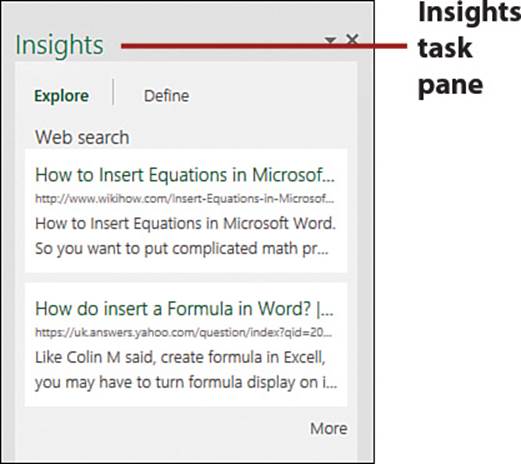
4. Select Smart Lookup to open the Insights task pane to view web-based information on the search term.
Making Selections from the Ribbon
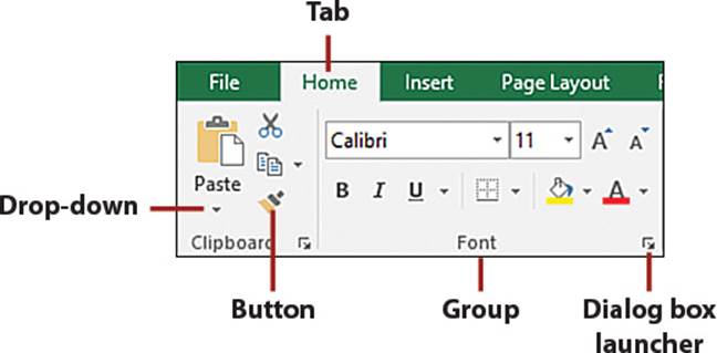
Along the top of the ribbon are tabs (labeled File, Home, Insert, Page Layout, Formulas, Data, Review, and View) that you can select to show options in the ribbon area below the tabs.
• Each tab consists of multiple groups containing buttons and drop-down menus.
• Clicking a button performs a function right away, such as bolding a cell or opening the Name Manager.
• Some buttons include arrows in the design. Clicking the main button area will perform the button’s default function, but clicking the arrow opens a drop-down with other options to choose from.
• Clicking a dialog box launcher opens up a dialog box with all the options of that group and more. If you can’t find the option you want on the group or you want to use multiple commands (for example, changing the font type and alignment of a cell’s contents), you might want to use the dialog box.
Customizing the Ribbon
If you’re working on a system with a small screen, the ribbon probably takes up too much space on the screen. You can minimize it or hide some tabs. Alternatively, perhaps you want a quicker way of getting to the ribbon options you use the most. In any case, Excel offers multiple customizations to make the interface handier for the way you use it.
Minimize the Ribbon Size
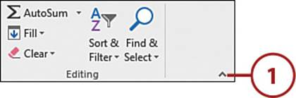
The ribbon can be minimized so that only the tabs are shown. When minimized, you can click the tab to temporarily view the tab’s controls.
1. Minimize the ribbon area by clicking the arrow in the lower-right corner of the ribbon.
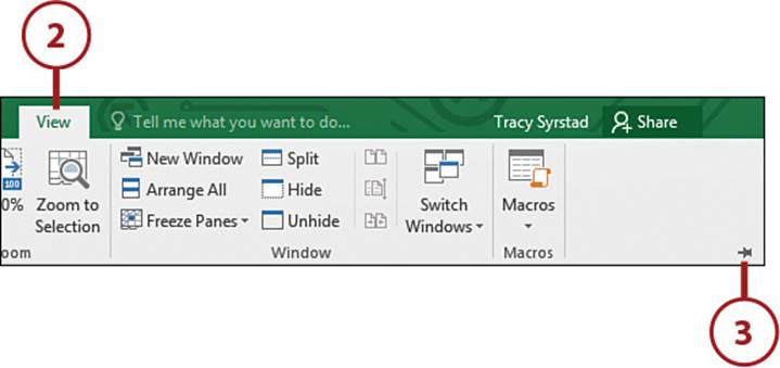
2. Open the ribbon back up by clicking any tab.
3. Lock the ribbon open by clicking the pin that now appears where the arrow used to be.
Toggling the Ribbon
To quickly toggle the ribbon between being minimized and normal (and locked), press Ctrl+F1 on the keyboard.
>>>Go Further: Ribbon Display Options
The Ribbon Display Options menu offers additional controls for showing and hiding the ribbon:
• Auto-hide Ribbon: This option completely hides the ribbon and the QAT, maximizing the sheet on your display. The Name box and Formula bar are still visible. When in this view, you can temporarily open the ribbon by clicking the three small dots in the top right corner of the screen. To hide the ribbon again, just click on the sheet.
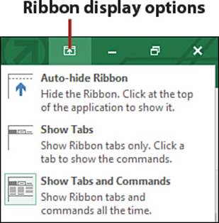
• Show Tabs: This option minimizes the ribbon in the same way as the steps outlined previously.
• Show Tabs and Commands: This option returns Excel to the default view showing all commands.
Add More Commands to the Ribbon
The default tabs and groups in Excel might not be the best ones for you or for a particular situation. You can insert a custom tab into the Main Tabs group or the Tool Tabs group. Once the tab has been added, you can add the commands most useful to you.
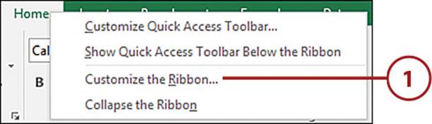
1. Right-click any tab and select Customize the Ribbon.
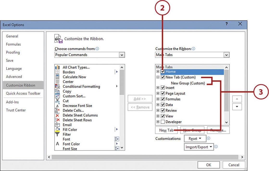
2. From the list on the right side of the dialog box, select where you want your tab to be. The new tab will be placed below and to the right of your selection.
3. Click New Tab. Excel creates a new tab with a new group, both with (Custom) after the name.
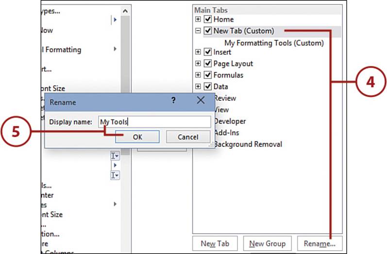
4. Click New Tab (Custom) and click Rename.
5. Type a new name in the Display Name field and click OK.
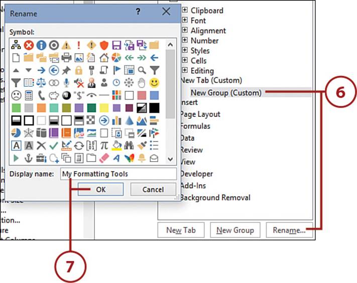
6. Highlight New Group (Custom) and click Rename.
7. Type a new name in the Display Name field and click OK.
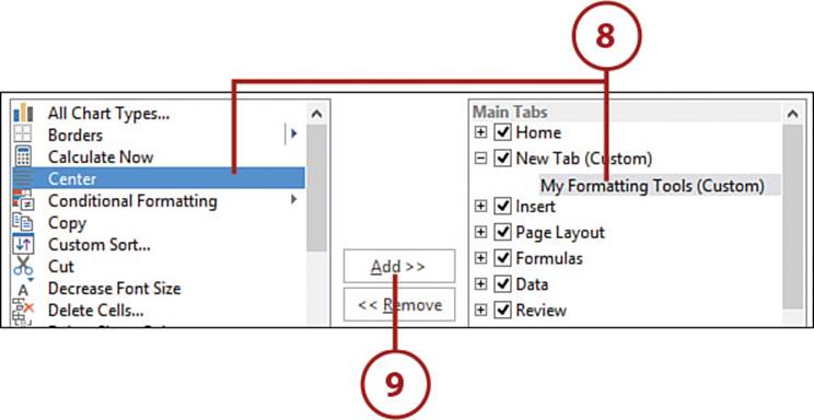
8. With the group to which you want to add a command selected, select the command you want to add.
9. Click Add.
Customize an Existing Tab
Excel won’t let you add a command to its existing groups. You can get around this by adding a custom group to an existing tab. Click the tab and add a new group by clicking the New Group button.
Customizing the QAT
The Quick Access Toolbar (QAT) is useful in that it doesn’t take up as much space as the ribbon, the commands don’t change based on what you’re doing, and you can customize it for a specific workbook.
Move the QAT to a New Location
By default, the QAT appears above the ribbon, but you can move it to below the ribbon.
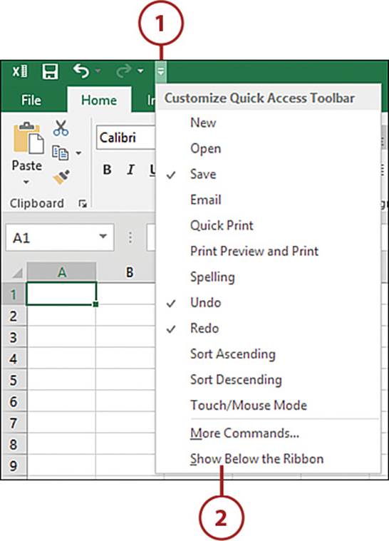
1. Click the arrow on the right end of the Quick Access Toolbar.
2. Select Show Below the Ribbon. If the toolbar is already below the ribbon, the option appears as Show Above the Ribbon.
Add More Commands to the QAT
Clicking the arrow on the right end of the QAT opens a list of commonly used commands. Click one of the options to add it to the QAT. If the command you want isn’t listed, you can select from the full list.
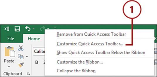
1. Right-click an existing command on the toolbar and select Customize Quick Access Toolbar.
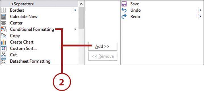
2. Select the desired command from the list and click Add.
Remove a Command
To remove a command from the QAT, right-click the command button you want to remove. Then, from the menu, select Remove from Quick Access Toolbar.
>>>Go Further: Customize the QAT for Just the Current Workbook
You can add commands to the QAT that will appear only when a specific workbook is open. To do this, select the workbook from the Customize Quick Access Toolbar drop-down on the right side of the dialog box.
Viewing Multiple Sheets at the Same Time
It’s easier to work on two sheets at the same time if you can view them simultaneously. If you have multiple monitors, you can drag one Excel window to another monitor. However, if you only have a single screen, you need to rearrange the windows to see them both.
Arrange Multiple Sheets
If you have multiple workbooks open, you can arrange the sheets so you can view them at the same time.
Compare Sheets of the Same Workbook
If you want to view multiple sheets of the active workbook at the same time, select View, New Window to create a duplicate window of the active workbook.
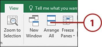
1. Click the View tab and then click the Arrange All button.
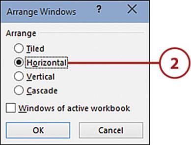
2. Select how you want to position the sheets (such as Horizontal) and then click OK.
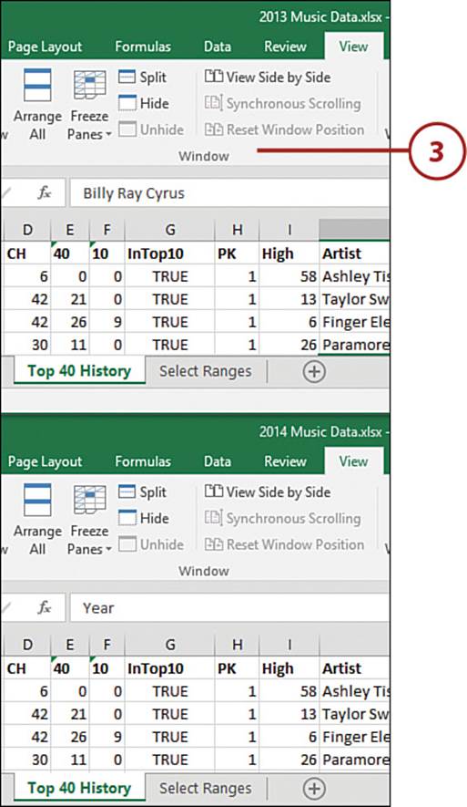
3. Excel will rearrange the windows of all open workbooks. To work in a specific window, click once anywhere on the sheet to activate it.
Scroll Two Sheets Side by Side
You can compare data row by row in two sheets by turning on Synchronous Scrolling.
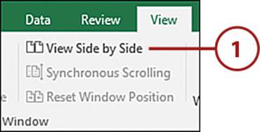
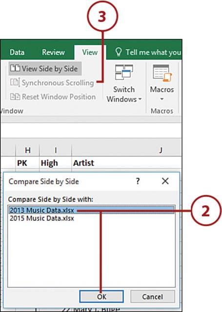
1. Click the View tab and then click the View Side by Side button.
Change Window Layout
If you don’t like the window positions after clicking the View Side by Side button, you can change them through the Arrange All tool. See the section “Arrange Multiple Sheets” for more information.
2. If you have only two workbooks open, Excel will arrange the two windows side by side. If you have more than two workbooks open, Excel will prompt for which window you want to use as the second one. Select the window and click OK.
3. Click the View tab and then click the Synchronous Scrolling button. As you scroll in one window, the other window will also scroll.
Changing the Zoom on a Sheet
The ability to zoom in and out on a sheet is an often-forgotten functionality in Excel. Instead, large fonts are used when a sheet is being designed, and then the designer later wonders why there are problems, such as the validation text being too small to see. Instead of relying on font size to make the text on the sheet larger, zoom in on the sheet. Excel offers several ways of changing the zoom on a sheet.
Use Excel’s Zoom Controls
Excel offers multiple methods for changing the zoom level of the active sheet.
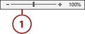
1. In the lower-right corner of the Excel window is the Zoom slider. Use the slider or the – and + buttons to change the zoom of the active sheet.
Or
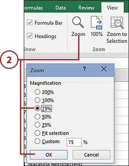
2. Click the View tab and then click Zoom. Select the desired magnification from the dialog box and then click OK.
Or
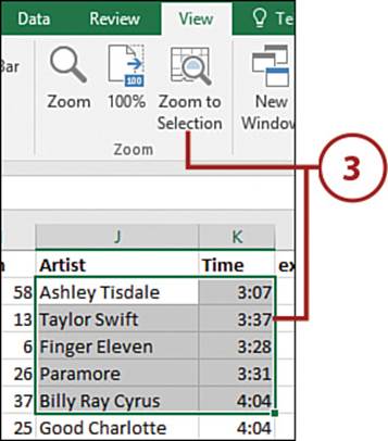
3. Select the range you want to zoom in on and then click View, Zoom to Selection.
Zooming with the Mouse
If your mouse has a wheel, you can use it to quickly zoom in and out on a sheet. While holding down the Ctrl key, spin the wheel on your mouse to change the magnification.
The magnification will focus on the active cell, keeping it always in view. So if there is a certain area you want to zoom in on, select a cell in that area first.
Moving Around on a Sheet
You can move around on a sheet using the mouse or the keyboard, depending on which method is most comfortable for you. To select a cell using the mouse, click the desired cell. To select a cell using the keyboard, use the navigation arrows on the keyboard. You can also use the number keypad arrows if the NumLock feature is turned off.
Keyboard Shortcuts for Quicker Navigation
Using the navigation arrows on the keyboard can be a little slow, especially if you have a lot of cells between your currently selected cells and the one you want to select. Even using the mouse can take some time to navigate from the top of your data to the bottom. The following list details a few keyboard shortcuts to make navigation a little easier:
• Ctrl+Home jumps to cell A1, located at the upper-left corner of the sheet.
• Ctrl+End jumps to the last row and column in use.
• Ctrl+Left Arrow jumps to the first column with data to the left of the currently selected cell. If there is no data to the left, a cell in the first column (A) will be selected.
• Ctrl+Right Arrow jumps to the first column with data to the right of the currently selected cell. If there is no data to the right, a cell in the last column (XFD) will be selected.
• Ctrl+Down Arrow jumps to the first row with data below the currently selected cell. If there is no data below the selected cell, a cell in the last row will be selected.
• Ctrl+Up Arrow jumps to the first row with data above the currently selected cell. If there is no data above the selected cell, a cell in row 1 will be selected.
Selecting a Range of Cells
To select a single cell, you click it once. However, you’ll often find yourself needing to select more than a single cell. For example, if you have text on a sheet you want to apply a new font to, instead of selecting one cell at a time and applying the font, you can select all the cells and then apply the font. When you have more than one cell selected, it’s called a range.
Where to Start
When you’re selecting a range, it doesn’t matter if you start at the top or bottom or the far left or far right of the range.
Select a Range Using the Mouse
Use the mouse to click and drag to select multiple cells.
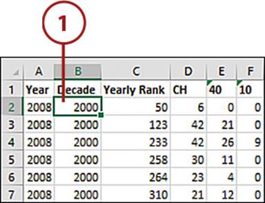
1. Select a cell that will be in the corner of your selection, such as B2.
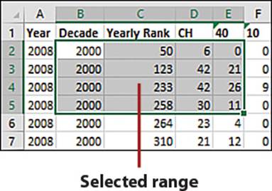
2. Hold down the mouse button as you drag the mouse to cover the desired cells.
3. When you get to the last cell, such as E5, let go of the mouse button. As long as you don’t click elsewhere on the sheet, the range will remain selected.
>>>Go Further: Use the Keyboard
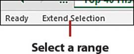
You can use the keyboard to select a range by turning Extend Selection mode on and off as needed. After selecting your starting cell, press F8 on the keyboard. The left side of the status bar shows Extend Selection mode is on. Use the keyboard to create your range and then press F8 again to stop the selection from extending. As long as you don’t select another cell, the range will remain selected. Refer to the previous section, “Keyboard Shortcuts for Quicker Navigation,” for shortcuts you can use to quickly select a range.
All materials on the site are licensed Creative Commons Attribution-Sharealike 3.0 Unported CC BY-SA 3.0 & GNU Free Documentation License (GFDL)
If you are the copyright holder of any material contained on our site and intend to remove it, please contact our site administrator for approval.
© 2016-2026 All site design rights belong to S.Y.A.