My Excel 2016 (2016)
10. Sorting Data
In this chapter, you’ll learn the various ways of sorting data, allowing you to view data from least to greatest, greatest to least, and even by color. You’ll also learn how to do the following:
→ Sorting data with one click
→ Sorting using a custom, non-alphabetical order
→ Sorting by color or icon
→ Rearranging columns with a few clicks of the mouse and keyboard
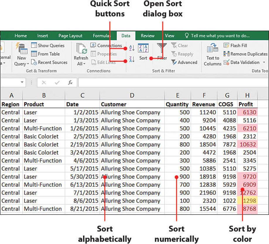
You’ll often need to sort your data, whether it be numerically, alphabetically, by color, or by icon. You aren’t limited to sorting the rows—columns can also be sorted.
Sorting data allows you to change how you view it. For example, if your dataset has a date column, you can view the oldest data at the top, or you can view the newest data at the top. You can also sort the data so like values, such as product names, are grouped together. You can even combine sorts so that you not only view the products grouped together, but in date order from oldest to newest.
Using the Sort Dialog Box
The Sort dialog box provides the most versatile way of sorting your data because it allows you to specify how you want the data sorted. When you use the dialog box, Excel applies each sort in the order it appears in the list.
Sort by Values
The Sort dialog box makes it easy to sort by multiple columns. A different sort method can be applied for each level. The sorts are done in the order they appear in the list.
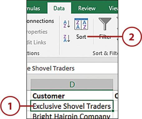
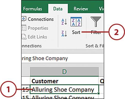
1. Select a cell in the dataset. Excel will use this cell to determine the location and size of the dataset.
2. On the Data tab, select Sort.
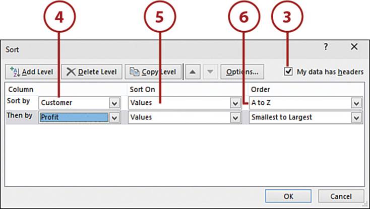
3. If the data has a header row, but Excel doesn’t recognize it, select the My Data Has Headers check box.
4. From the Sort By drop-down, select the first column header by which to sort.
5. From the Sort On drop-down, select Values.
6. From the Order drop-down, select the order by which the column’s data should be sorted. Choose A to Z to sort in alphabetical order; choose Z to A to sort in the opposite order. If the data is numerical, the drop-down options will change to Smallest to Largest and Largest to Smallest.
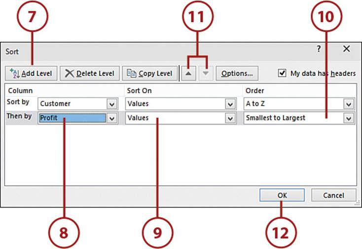
7. Select Add Level to add another sort rule.
8. From the Then By drop-down, select the second column header by which to sort.
9. From the Sort On drop-down, select Values.
10. From the Order drop-down, select the order by which the column’s data should be sorted.
11. If you realize a field is in the wrong position, use the up or down arrow at the top of the dialog box to move the field to the correct location.
12. Click OK to sort the data.
It’s Not All Good: Excel Didn’t Select the Dataset Correctly
When you sort, Excel will try to help by selecting your dataset for you. You can help Excel do this correctly by not having any blank rows or columns in your dataset. Also, ensure that your header, if you have one, consists of only one row. Only a single header row is allowed—any rows after it are treated as data.
If Excel incorrectly selects your data, exit from the Sort dialog box, delete the blank columns and rows, and start the dialog box over.
If for some reason you can’t delete the blank columns or rows, you can pre-select the entire table before starting the Sort dialog box.
Sort by Color or Icon
Excel can also sort data by fill color, font color, or an icon set from conditional formatting.
1. Select a cell in the dataset. Excel will use this cell to determine the location and size of the dataset.
2. On the Data tab, select Sort.
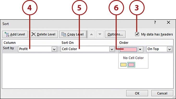
3. If the data has a header row, but Excel doesn’t recognize it, select the My Data Has Headers check box.
4. From the Sort By drop-down, select the column header by which to sort.
5. From the Sort On drop-down, select Cell Color to sort by the cell’s fill color. You can also choose Font Color to sort by the value’s color or Cell Icon to sort by conditional formatting icons.
6. From the first Order drop-down, select the color by which the column’s data should be sorted. If sorting by icon, you’ll have a choice of icons.
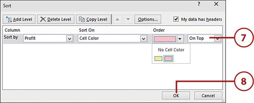
7. From the second Order drop-down, select whether the color should be sorted to the top or bottom of the data. If you select multiple colors to sort at the top of the data, the colors will still appear in the order chosen.
8. Click OK to sort the data.
Color Sorting a Table
If your data is in a table, you don’t have to go through the Sort dialog box. Instead, click the arrow in the header, select Sort by Color, and select the color you want sorted to the top of the table.
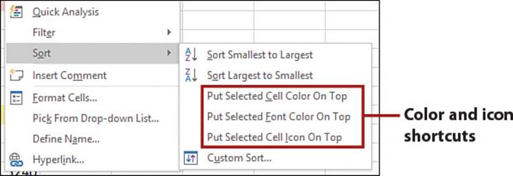
>>>Go Further: Sorting Shortcut
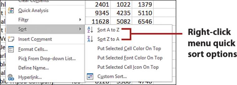
In addition to sorting colors and icons through the Sort dialog box, the following options are also available when you right-click a cell and select Sort from the context menu.
If you use one of the preceding options to sort more than one color or icon, the latest selection will be placed above the previous selection. So, if yellow rows should be placed before the red rows, sort the red rows first, and then the yellow rows.
Doing Quick Sorts
The Quick Sort buttons offer one-click access to sorting cell values.
Quick Sort a Single Column
There are several quick methods you can choose from to apply simple sorts to your data.
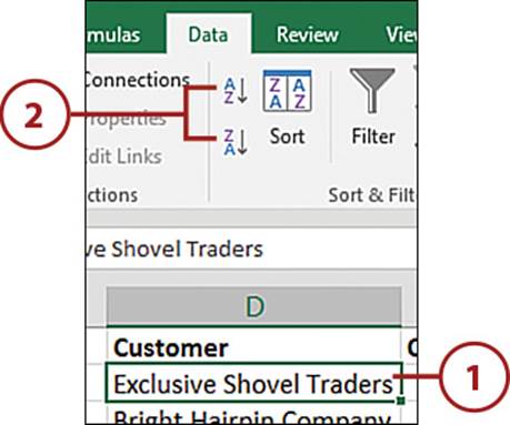
1. Select one cell in the column to sort by. If you select multiple cells, Excel will sort only the data in the selected range.
2. On the Data tab, select AZ to sort lowest to highest or ZA to sort highest to lowest.
>>>Go Further: Other Quick Sort Options
There are other ways you can access the quick sort options:
Right-click the cell and select Sort, Sort A to Z or Sort Z to A if your data is text; select Sort Smallest to Largest or Sort Largest to Smallest if the data is numerical.
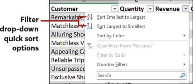
From a filter drop-down, select Sort A to Z or Sort Z to A if your data is text; select Sort Smallest to Largest or Sort Largest to Smallest if the data is numerical.
Settings Carry Between Sorts
Sort options are retained for the sheet during an Excel session. So if you set up a custom sort with Case Sensitive turned on, then later do a quick sort, the quick sort will be case sensitive.
Quick Sort Multiple Columns
If you keep in mind that Excel keeps previously sorted columns sorted as new columns are sorted, you can use the Quick Sort feature to sort multiple columns. For example, if the Profit column is organized, Excel doesn’t randomize the data in that column when the Customer column is sorted. Instead, Profit retains its order to the degree it falls within the Customer sort. The trick is to apply the sorts in reverse to how they would be set up in the Sort dialog box.
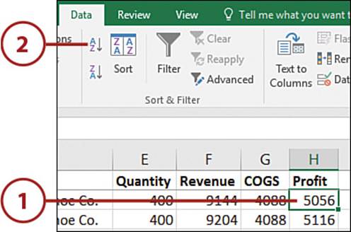
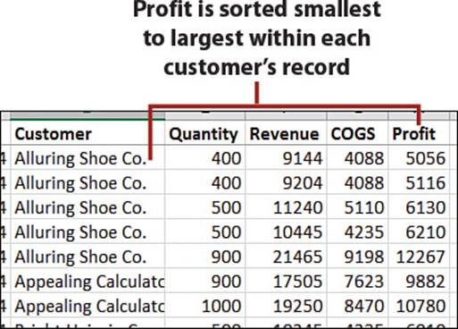
In the following example, we want to sort by Customer and Profit, both least to greatest.
1. Select a cell in the column that should be sorted last in the Sort dialog box (in this case, the Profit column).
2. On the Data tab, click the A to Z button.
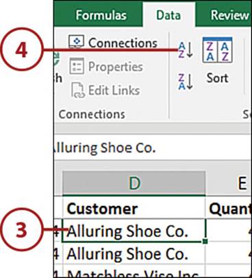
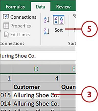
3. Select a cell in the next column to be sorted (in this case, the Customer column).
4. On the Data tab, click the A to Z button.
5. The table is now sorted by Customer and then Profit within each customer’s records.
Performing Custom Sorts
You aren’t limited to sorting data alphabetically and numerically. With a little extra setup work, you can randomize the order or sort by a custom sequence.
Perform a Random Sort
Excel doesn’t have a built-in tool to do a random sort, but by using the RAND function in a column to the right of the data and then sorting, you can create your own randomizer.
1. Add a new column to the right of the data and give the column a label in the first cell, such as Random.
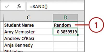
2. In the second cell of the new column, type =RAND() and press Ctrl+Enter (this will keep the formula cell as the active cell). The formula will calculate a value between 0 and 1.
3. Copy the formula to the rest of the rows in the column.
4. Select one cell in the new column.
5. On the Data tab, click the AZ button.
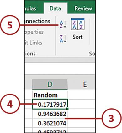
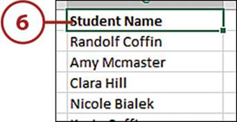
6. The list will be sorted in a random sequence. Delete the temporary column added in step 1.
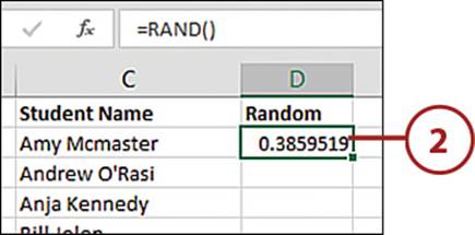
The Numbers Keep Changing
Right after Excel performs the sort, it recalculates the formula in the temporary column, so it may appear that the numbers are out of sequence.
Sort with a Custom Sequence
At times, data may need to be sorted in a custom sequence that is neither alphabetical nor numerical. For example, you might want to sort by month, by weekday, or by some custom sequence of your own. You can do this by sorting by a custom list.
How to Create a Custom List
You’ll need to create a custom list before continuing with the following steps. Refer to “Create Your Own List” in Chapter 4, “Getting Data onto a Sheet,” for steps on creating one.
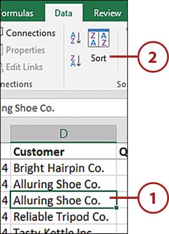
1. Select a cell in the dataset.
2. On the Data tab, click Sort.
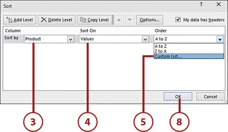
3. From the Sort By drop-down, select the column header by which to sort.
4. From the Sort On drop-down, select Values.
5. From the Order drop-down, select Custom List.
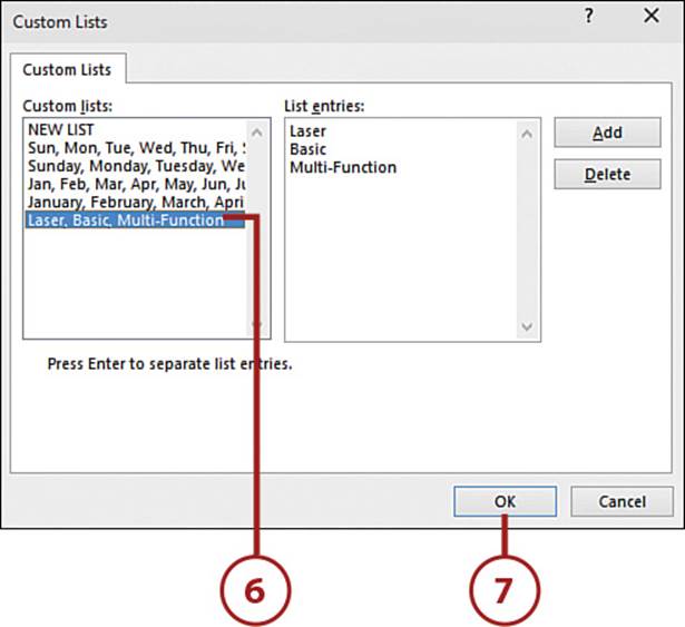
6. Select the desired list.
7. Click OK.
8. Click OK.
9. The data is sorted by the custom list.
Rearranging Columns
By default, data is sorted by rows, but you can choose to sort columns instead. And with the following trick, you aren’t limited to sorting them alphabetically.
Sort Columns with the Sort Dialog Box
Hidden in the Sort dialog box is an option to sort your data left to right, instead of the default top to bottom.
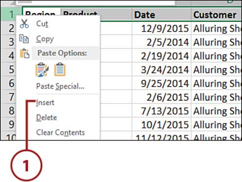
1. Insert a new blank row above the headers by right-clicking the row 1 heading and then selecting Insert.
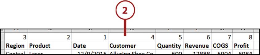
2. In the new row, type numbers corresponding to the new sequence of the columns, with 1 being the leftmost column, then 2, 3, and so on, until each column has a number denoting its new location.
3. Select a cell in the dataset.
4. Press Ctrl+A to select the current region, including the two header rows.
5. On the Data tab, select Sort.
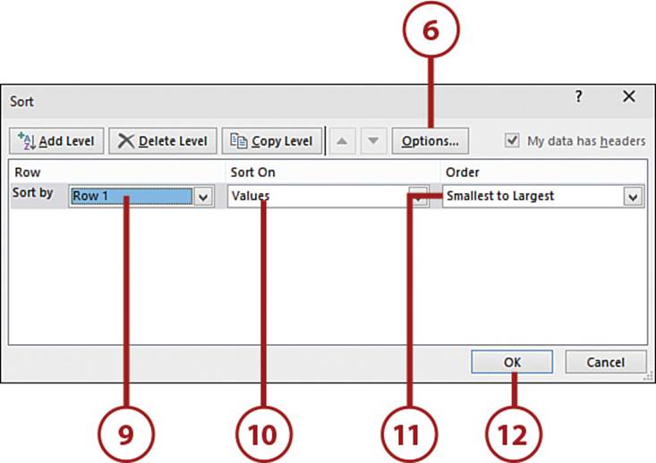
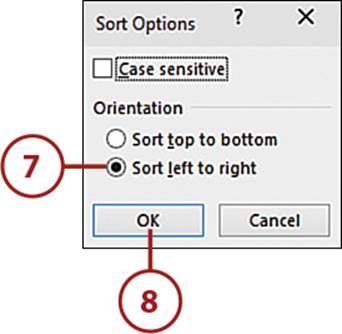
6. Click the Options button.
7. Select the Sort Left to Right option.
8. Click OK to return to the Sort dialog box.
9. In the Sort By drop-down, select Row 1.
10. In the Sort On drop-down, select Values.
11. In the Order drop-down, select Smallest to Largest.
12. Click OK.
13. Excel will rearrange the columns.
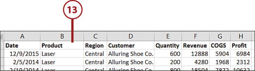
14. Delete the temporary row added in step 1.
Fixing Sort Problems
If it looks like the data did not sort properly, refer to the following list of possible solutions:
• Make sure no hidden rows or columns exist.
• Use a single row for headers. If you need a multiline header, either wrap the text in the cell or use Alt+Enter to force line breaks in the cell.
• If the headers were sorted into the data, there was probably at least one column without a header.
• Column data should be of the same type. This may not be obvious in a column of ZIP codes where some (such as 57057) are numbers, but others that start with zero are actually text. To solve this problem, convert the entire column to text.
• If you’re sorting by a column containing a formula, Excel will recalculate the column after the sort. If the values change after the recalculation, such as with RAND, it may appear that the sort did not work properly, but it did.
All materials on the site are licensed Creative Commons Attribution-Sharealike 3.0 Unported CC BY-SA 3.0 & GNU Free Documentation License (GFDL)
If you are the copyright holder of any material contained on our site and intend to remove it, please contact our site administrator for approval.
© 2016-2026 All site design rights belong to S.Y.A.